ECHAM-MPI model runs, Ocean Heat Content, and Katsman and van Oldenborgh 2011

As I mentioned in my last post, the GISS-ER projections for ocean heat content did not seem to include any period of flattening like we’ve seen between 2003 and the present, so I wanted to see if some other CMIP3 models might include the variability in upper ocean heat content to explain such observations.  Over at Real Climate, Dr. van Oldenborgh mentioned that his paper (I’ll call it KO2011 from here on out) used 17 runs from ECHAM-MPI to explain the current flattening.  The three key points for the paper listed at GRL are:

• An 8-yr period without upper ocean warming is not exceptional
• It is explained by more radiation to space (45%) and deep ocean warming (35%)
• Recently-observed changes point to an upcoming resumption of upper ocean warming

First, I will note that the projections (these start in 2001) for the upper 700m DO seem to show more variability than GISS-ER, (despite there only being 2 for the SRESA1B scenario at PCMDI) which is a good thing when it comes to explaining the recent flattening:

I’ve once again baselined to the overlapping years, which now starts in 2001.  As you can see, it still seems like ECHAM-MPI has difficulty reproducing the variability, but it is not quite as monotonic as GISS-ER. 

However, while the Katsman and van Oldenborgh paper does some interesting analysis with respect to deep ocean warming and the model simulations, there are a few problems with it that lead me to question those three key points. 

Issue #1 – A Statistical Problem of Independence

In KO11, they use 17 different runs, and then calculate all of the different overlapping 8-yr trends during the period for each of the runs, yielding their following conclusions:

From the distribution of linear trends in UOHC, it appears that 11% of all overlapping 8-yr periods in the time frame 1969–1999 have a zero or negative UOHC trend (Figure 2a). Over 1990–2020, around the time of the observed flattening, this is reduced to 3% (Figure 2b), corresponding to a probability of 57% of at least one zero or negative
8-yr trend in this time frame.

Bold mine.  The 3% actually appears to be rounded up from 2.66%, which is calculated by 14 of these overlapping 8-year trends from "17 members × 31 overlapping 8-yr periods = 527 trend values" having seen a trend of 0 or negative.  The 57% percent could then be calculated based on the probability that 31 of the non-events do NOT occur, or 1- (1 – .0266)^31 = 57%.  Clearly, there appears to be a problem.  These event are treated as independent, when clearly the fact that the trends are from overlapping periods means there will be high amounts of autocorrelation (quite separate from year-to-year OHC exhibiting autocorrelation).  In other words, it ignores the fact that a particular ensemble member containing one negative 8-year trend is more likely to have another 8-year trend (particularly if 7 of those years are overlapping) that is negative, so that the probability of any particular run having "at least one zero or negative 8-yr trend in this time frame" is actually substantially less than that 57%.

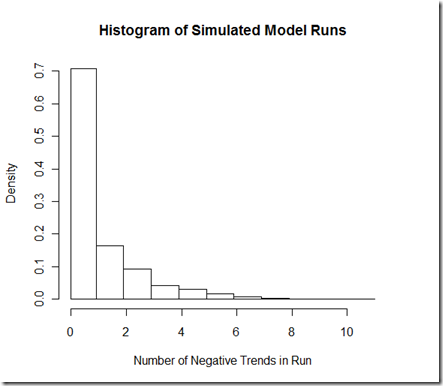
The degree to which it is different I believe depends largely on the autocorrelation/noise model.  I’ve used a ARIMA(2,0,2) for the noise, which I got as a "best fit" from one of the ECHAM-MPI runs, and added in a trend for this simulation.  I’ve tuned to model to give approximately the 2.66% negative trends presented in the paper.  Anyhow, running the simulation 1000 times yields 797 negative 8-yr trends out of (1000 runs * 31 8-yr periods) or 2.57% of the trends are negative.  By the logic in KO11, we should expect that there is a 55% chance [1-(1-.0257)^31] that we’d see a negative trend over any given run.  However, if we look at our simulation, only 36% (362 out of 1000) of the runs actually contain the negative trend.  A look at our histogram below shows why:

Out of the 362 runs that contain at least one negative trend, a whopping 197 of them contain 2 or more negative trends, far more than we would expect if they were independent trials, but quite what we’d expect with these overlapping periods. 

But really, much of this extra simulation is unnecessary.  A look at figure 2b seems to show (if I’m reading the colors correctly) that 5 out of the 17 ensemble members during this period show a zero or negative trend, or 29%.  Yes, this is a smaller sample size, but if KO11 had simply reported this they would have avoided this statistical pitfall, and the 29% is almost certainly a more correct figure than the 57%.  Figure 2B from KO11 (each color represents a different member of the ensemble):

Does this issue "matter"?  On the one hand, I would argue that yes, it matters if the probability of this happening over the 31-year period is more likely than not (57%) vs. less than a 1 in 3 shot.  On the other hand, using a length of 31 years to diagnose whether an 8-yr event is "exceptional" seems rather arbitrary, particularly when it happened right after the SRES projections began.  Furthermore, why KO11 also prominently included the 1969-1999 centered 8-year trends (which includes 1966 as the first year) is a mystery to me, given that the change in anthropogenic forcings used for the model over that period do not resemble the magnitude present in estimates for the 2003-2010 period.  I’m not quite sure how to interpret the "not exceptional" part: certainly, if I can choose a model with some of the highest variability, choose a length of time for the event to happen, and/or choose a period with a smaller increase in forcings, then run this model numerous times, it seems possible that the event may occur with likelihood over that period.  When it comes to examining the CMIP3 models as a whole, I might ask what percentage of the ensemble members showed an OHC trend resembling that 2003-2010 period?  I won’t know until I process all the different runs for the different models.

Issue #2 – The ENSO observations do not bear out the theory

From KO11, under the "Recent Absence of Ocean Warming" section, we read:

During 2002–2007, a series of El Niño events occurred (www.cpc.noaa.gov/data/indices/), which probably yielded a larger than average upper ocean heat loss [Trenberth et al., 2002] caused by the (lagged) response through net outgoing TOA radiation (Figure 3b). This seems at odds with direct observations that indicate an opposing increase in the radiation from space [Trenberth and Fasullo, 2010], but the record has large uncertainties and is too short to separate trends from decadal variability.

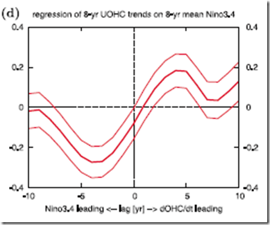
KO11 readily admit that the TOA radiation observations do not match the behavior in the models that explain the flattening of UOHC, but chalk this up to uncertainties and a short record.  That’s fine.  But the comment about 2002-2007 "El Nino events" seems to make little sense given the theory that has been established throughout the paper.  Basically, KO11 show that in the model simulations, El Nino events result in a heat loss that leads to a decrease in the ocean heat content trend in subsequent years, whereas La Ninas have the opposite effect (heat gain) and lead to an increase in the OHC trend.  A very specific lagged correlation is shown between the mean Nino3.4 index over an 8-year interval and the 8-year OHC trend in figure 3d:

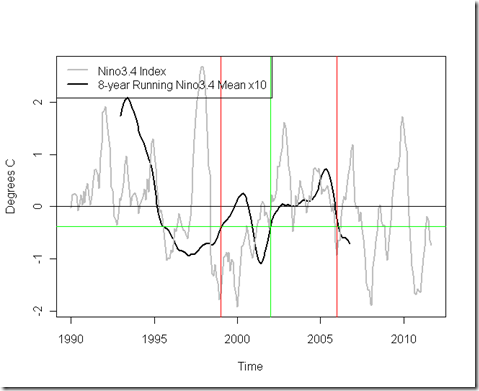
According to the graph of theory/model simulations, the OHC trend from 2003-2010 would be driven by the mean 8-year Nino3.4 index from 4 years prior, or 1999-2006 (that is, the running mean centered on 2002).  Below, I’ve shown the Nino3.4, with this relevant portion highlighted:

The two red lines bound the ENSO period we’re talking about, and the green lines point to the specific point in the running mean that would be relevant according to the theory.  Note that in 2002 it is actually BELOW 0, closer to La Nina conditions, which is the opposite of the strong decadal El Nino (positive Nino3.4 index) that the theory projected would have caused such a flattening!  Yes, we see El Ninos between 2002-2007, but we also see a lot of fluctuations in the opposite direction…that’s the nature of ENSO.  However, unless I’ve missed something (which is quite possible), or the chart is unclear, I cannot see how the combination of the flattening OHC trend and the observed Nino3.4 is at all consistent with the model findings, and in fact seems to contradict them. 

So does this issue matter?  In this case, I think the answer is “yes”.  The current OHC trend would seem to be exceptional according to the model, if we experienced it without the corresponding ENSO variation that would have been expected to cause the extra 45% heat to radiate to space.  Furthermore, the  projection of an “upcoming resumption of upper ocean warming” depends largely on the shift in ENSO to La Nina conditions, but, as we’ve seen, the La Nina conditions already were present 4 years prior to the current flattening.  If I had to bet, I would bet that OHC warming indeed picks up again, but this particular attribution to ENSO does not seem to have much observational support.

Anyhow, all code and intermediate data for this post can be found here.