Changes in feedback strength with time: a look at the 1pct2xCO2 GFDL CM2.1 experiment

In this half-baked post, I want to look a bit more at the issue of how the radiative response (λ) in our familiar equation (ΔN = ΔF + λ*ΔT) changes as we progress through the 1% CO2 increase per year to doubling experiment in GFDL CM2.1.  As we’ve discussed before, this issue makes it extremely difficult to diagnose equilibrium climate sensitivity (ECS) in models even if we have 100 years of the exact global energy balance observations. The "effective sensitivity" (λ after 100 years in the A1B scenario, per the label in Soden and Held (2006)) when used in the equation F_2xCO2 / λ , may yield an ECS that is greater or lower than the actual ECS of the model.  Examples of the two extremes in CMIP3 (per Winton et al. 2010): 

1. For MPI-ECHAM5, "effective sensitivity" λ = -0.88 W/m^2/K, F_2xC02 = 4.01 W/m^2, yielding ECS (assuming constant λ) of 4.01/0.88 = 4.6 K, compared to the actual ECS 3.4 K.
2. For GFDL CM2.1, "effective sensitivity" λ = -1.37 W/m^2/K, F_2xCO2 = 3.5 W/m^2, yielding ECS (assuming constant λ) of 3.5/1.37 = 2.6 K compared to the actual ECS of also 3.4 K.

But really, the issue is more than just about whether λ after 100 years matches the "final" value for λ from a CO2 doubling.  In the real world, we have far less data relevant to the Earth’s energy balance (a little over a decade of continuous satellite measurements, with OHC extending back further, as I used previously), so knowing how the radiative response (λ) changes with time and temperature would be crucial for diagnosing longer-term sensitivity.  Again, I will recommend the Paul_K post on the Blackboard and Isaac Held’s post or more in-depth background. 

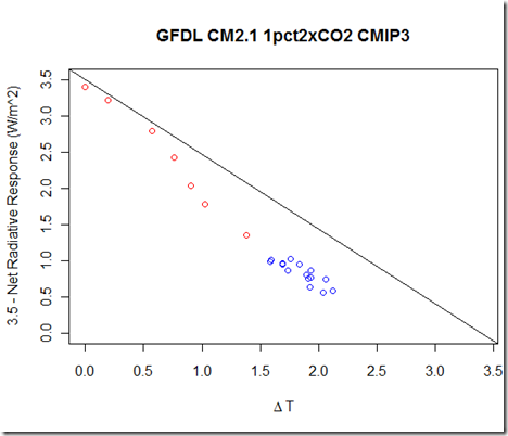
Unfortunately, from the CMIP3 archive, only 220 years of the 1% increase to CO2 doubling is available, which is far from the time it takes to achieve equilibrium.  Nevertheless, by plotting the CO2 doubling forcing (3.5 W/m^2 in CM2.1) minus the radiative response to T (very similar to Dr. Held’s graph in that post), we can still see that λ (the relationship between the radiative response and T) is not a constant, as the values plotted drop below the "constant λ" (3.5/3.4 = 1.03 W/m^2/K) line. 

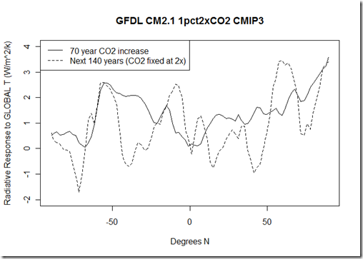
I wanted to explore a case for the apparent non-linearity in the global radiative response strength being the result of differing spatial patterns in the surface temperature changes in different time frames.  Let’s suppose that the surface temperature change in each latitude band affects almost exclusively only the outgoing radiation over that same latitude band, such that dR_lat/dT_lat is a constant value.  Potentially, we could get an apparent non-linearity in the global radiative response if the relative rate of heating at different latitudes changes.  This is actually an extremely simplified scenario of the more general situation described by Dr. Held.  Unfortunately, my simplified case here does not hold:

    
Clearly, there are significant changes in dR_lat/dT_lat over the two periods.  This is NOT to say that the differential warming pattern alone isn’t responsible for the apparent non-linearity, but rather that surface temperatures at one latitude must significantly affect the TOA imbalance at another latitude (circulation and cloud changes) or the spatial pattern within a particular latitude must be important, if we are to maintain this idea.  It is possible that using broader regions (rather than single latitude bands) could better capture this, which I will explorer in the future.  

Here is how each latitude warms per 1 degree of global increase in the differing periods:

And for reference, in those periods, here is what the radiative response strength looks like relative to the global temperature increase:

Northern vs. Southern Hemisphere Warming

While looking at this experiment, I also want to harken back to a previous post on the NH vs. SH rate of warming.  Here is how the two hemispheres warm in this experiment:

 

The ratio of NH to SH trends for 30, 50, 100, and 220 years respectively are 2.2, 1.3, 1.3, and 1.5.  This would seem to suggest that, at least in this model, it is unlikely that GHG would account for the ratio of around 3.3 we have seen in recent GISS temperatures, particularly given that aerosols produce the stronger negative influence in the NH.

Code and data (you’ll need to download the runs from PCMDI)