Troy's Scratchpad

October 30, 2014

Combining recent instrumental sensitivity estimates with paleo sensitivity estimates

Filed under: Uncategorized — troyca @ 7:46 pm

In the last couple years, there have been quite a few papers using the instrumental period to estimate equilibrium*** sensitivity, with most of them finding best estimates heavily concentrated near the lower end of the IPCC 1.5K – 4.5K assessed "likely" range.  Examples include Aldrin et al. (2012), Ring et al. (2012), Otto et al. (2013), Lewis (2013), Skeie et al. (2014), Masters (2014), Loehle (2014), and, more recently, Lewis and Curry (2014).  I think this general theme stems from a few factors: 1) the lower-than-expected increase in surface temperatures at the turn of the century, 2) a decrease in estimates of the magnitude of the anthropogenic aerosol cooling offset, and 3) more constrained estimates of OHC in recent years.

Many people argue that these studies indicate that sensitivity is less than previously thought, and that policies and risk analysis should reflect the downgraded estimates.  Critics, on the other hand, often point to paleo evidence to dismiss the impact of these studies on our current expectations of CO2-induced warming.  Therefore, I thought it would be interesting to combine the latest estimates of sensitivity from PALAEOSENS (2012), which I take to represent synthesized evidence from paleo estimates, with my (admittedly ad-hoc) synthesized evidence from a few of these recent instrumental era estimates with published distributions.  This Bayesian approach of combining different lines of independent evidence is nothing particularly new, having been done by Annan and Hargreaves (2006), but I was curious to see how it would shake out with these recent estimates.  Here are the results:

combined_sensitivity

Numerically, the result of the “combined” evidence is a median of 2.1 K, a “likely” (68%) range of 1.5-2.9 K, and a “very likely” (95%) range of 1.1K-3.9K.  There are a few caveats here: first, I used WebPlotDigitizer to quickly digitize the values from the aforementioned studies, which is a nifty tool, but obviously not perfect.  Second, your results for this kind of method are always going to be affected by the studies chosen, although I think the “Instrumental Mean” line – with its mode and median between 1.5 and 2.0 K – is probably a fair representation of the evidence from these type of studies.  And finally, it could be argued that there are structural uncertainties in our knowledge that permeate both the paleo and instrumental estimates, such that these lines are not truly “independent”, and the resulting uncertainty ranges should be wider. 

Script for this post can be found here.

***these methods range from assuming effective=equilibrium sensitivity (e.g. Otto et al 2013) to explicitly considering the modeled differences (e.g. Masters 2014).  

September 3, 2014

CMIP5 processing on Github, with another comparison of observed temperatures to CMIP5 model runs

Filed under: Uncategorized — troyca @ 7:05 pm

I recently started a small library of functions I use frequently to process downloaded CMIP5 runs on Github.  Additionally, there are some processed files I uploaded to that repository, which are the monthly global tas (surface air temperature) text files for a large fraction of available CMIP5 runs. 

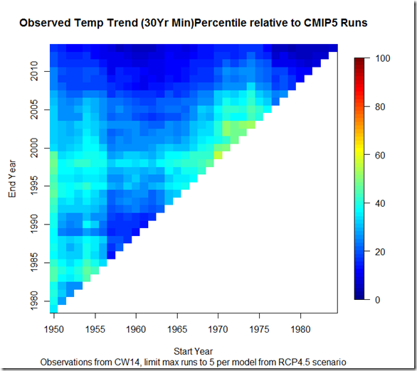
In order to put these to use, I thought it would be interesting to investigate where the “observed” temperature trend appears relative to all CMIP5 runs for every combination of start and end years from the last half of the 20th century (1950) to present (2013).  Thus, below I show the “percentiles”, where red values indicate the observed temperature trend is running hot relative to the models (75th percentile means the observed trend is larger than 75% of the model runs over that same period), and blue indicates the observed temperature trend is running cool relative to the models.

The list of models included can be found here.  In order to avoid too strongly overweighting certain models relative to others, I have restricted the number of runs to include per model to a maximum of 5.  The temperature observations come from the Cowtan and Way (2014) kriging of HadCRUTv4.  Here is the result if we look at all trends over this period that span 15 years or more:

observedAndModeled15yr

From a glance, it appears that there is a good deal more blue than red here, suggesting that a lot of the observed trends are running towards the cooler end of models.  Some recent papers (eg. Risbey et al (2014) ) have been looking at the “hiatus”, and in particular 15 year trends, arguing that the most recent low 15 year trend doesn’t necessarily provide evidence of oversensitive CMIP5 models because these models cannot be expected to simulate the exact phasing of natural variation.  They point out that at points in the past, the observed 15 year trends have been larger than that of the models.  There is some support for that in the above graph, as shorter trends ending around 1970 or in the 1990s tended to be towards the higher end of model runs.  Moreover, I think that anybody suggesting that the difference between observed and modeled trends during the “hiatus” was due solely  to oversensitivity in models is misguided.

That being said, I think if we move past the “models are wrong” vs. “models are right” dichotomy and onto the “adult” question of “are models, on average, too sensitive in their transient responses?” we can agree on the following: given the apparent large contribution of internal variability to 15 year trends, seeing these observed trends in both the upper and lower percentiles of modeled trends is to be expected, even if models on average were too sensitive in the transient by, say, 35%.  In the case of models being too sensitive, we would simply expect to see more trends in the lower percentiles than higher percentiles, as above. 

However, I think a more striking picture emerges if we look at only 30-year or longer trends, where some of the higher frequency variations are filtered out:

observedAndModeled30yr

Here, we see that depending on start and end year picked, the observed trends generally fluctuate between the 2nd and 50th percentiles of model runs.  This seems to be strong evidence that the CMIP5 runs are, on average, running too hot.  Otherwise, one might expect the observed trends to fluctuate more evenly above and below the 50th percentile.  Whether they are running too hot because of incorrect forcings or oversensitivity cannot be divined from the above figure, but I think it provides stronger evidence that the models are running warm than the single most recent 15-year period. 

Script available here.

June 13, 2014

Estimating ECS bias from local feedbacks and observed warming patterns–example with GFDL-CM3

Filed under: Uncategorized — troyca @ 10:45 pm

1. Introduction

Typical energy balance methods, such as Otto et al (2013) or Masters (2014), have been frequently used for estimating equilibrium climate sensitivity (ECS) over the instrumental period.  Recently, several studies have raised the possibility that these may be biased, even if one were to precisely pin down the magnitude of the aerosol forcing and the current top-of-atmosphere (TOA) energy imbalance. In particular, the net feedback or radiative restoration parameter (typically represented by lambda) may be different when calculated over the instrumental period vs. the long-term, idealized CO2-only simulations.  One could partition this into two factors:

1) Inhomogenous Forcings. Certain forcings, such as aerosols, may be concentrated in higher-latitude regions, where the net feedback is smaller, thereby “cancelling out” more of the homogenous greenhouse forcing when looking only at the globally-averaged TOA imbalance.  This was raised recently in the Kummer and Dessler (2014) extension of the Shindell (2014) forcing “enhancement” from TCR to ECS (although as discussed previously, the enhancements in TCR and ECS are very different).

2) Time-Varying Sensitivity. Armour et al (2013) suggest that this may result from time-invariant local feedbacks, with only the spatial warming pattern changing over time and triggering these local feedbacks in changing proportions over time.

In fact, if we take the Armour et al (2013) view, both #1 and #2 have the same root cause – the differing spatial warming pattern between the transient, instrumental warming pattern case, and the long-term idealized 2xCO2 scenarios run in the models. 

2. Method 

If you will recall, one of my criticisms of Shindell et al (2014) was that it did not consider the observed spatial warming pattern.  Essentially, when determining forcing enhancements, it relied on the GCM output for:

a)  The ratio of the localized temperature response relative to the global response (essentially the relative heat capacity of each region)

b) The spatial warming pattern in the idealized GHG scenarios

c) The spatial warming pattern over the historical/instrumental period

While a and b may need to be relied upon, it seems as though one could use the information from c during the observed instrumental period, rather than relying on something that GCMs do poorly (regional warming projections, response to aerosols, and horizontal heat transfer).  Moreover, an ensemble of runs from a GCM will not be able to reproduce the exact variability seen in the single “realization” of the instrumental period.  To me,  it seems more likely that GCMs might be more correct and agree better on a and b than they would on c.  But even if they are not, at least it is one less assumption that needs to be made regarding GCM accuracy. 

By analogy, I think there is a reasonable method for determining the bias in ECS when calculated over the instrumental period.  Essentially, for different GCMs, we would calculate

a) The zonal net feedback according to the GCM.  We do this by first calculating the forcing for each zone using the difference in TOA imbalance for the last 25 years of the fixedSST regressions: sstClim4xCO2 – sstClim.  Then, for each zone we calculate the difference in TOA balance between the abrupt4xCO2 experiment and the piControl experiment, subtract the forcing calculated in the prior step, and normalize this by the local temperature increase calculated as the difference between abrupt4xCO2 and the piControl.  Note: this relies on the assumption of Armour et al (2013) that the increase in surface temperature in one region primarily affects the outgoing radiative response locally, rather than over some other area. At the end, we have an n x 1 column vector A,  with n being the number of zones.

b) The spatial warming pattern over the idealized scenario from the GCM that we will use as a baseline.  For example, if one were interested in how inhomogenous forcings may create a bias in energy balance estimates over the instrumental period, one might use the historicalGHG or abrupt4xCO2 scenario over a time period similar to the length of the historical period.  If, on the other hand, one wanted to figure out the combined effect of those inhomogenous forcings + time-varying sensitivity, one would use the spatial warming pattern of a run that had achieved radiative equilibrium after a doubling of CO2.  Regardless, we calculate an n x 1 column vector B, which consists of each of zone’s temperature change, normalized by the global temperature change.

c) The observed spatial warming pattern.  Similar to the step above, we calculate an  n x 1 column vector C, which consists of each zone’s observed  temperature change over the instrumental period, normalized by the total global temperature change.

Finally, we can then calculate what the expected bias in net feedback calculated over the instrumental period will be, according to each model, using the following equation:

Eq. 1 

Where the function “weight” simply multiplies each element in the vector by its area fraction of the globe.

3. Example with GFDL-CM3

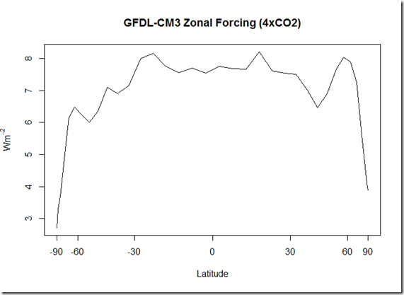
First, here is the fixed-SST forcing calculation:

GFDL_CM3_Zonal_Forcing

One thing of interest here is that the global forcing actually comes out to 7.2 W/m^2 for 4xCO2, which is more in line with the typical value of 3.7 W/m^2 for a doubling of CO2, and well above what is calculated in Andrews et al (2012) using the regression technique.  However, a look at figure 1 from Andrews et al (2012) highlights why:

andrews_et_al2012_gfdl_cm3

As you can see, there is one point with a net imbalance above the intercept at 6 W/m^2 which Andrews et al (2012) takes as the forcing.  Clearly, since the regression is affected greatly by the larger T points and there is significant curvature, the regression method in this case underestimates the forcing.

Moving on, here is the calculation of the zonal net feedbacks:


GFDL_CM3_Zonal_Feedback

Interestingly, this seems to differ from the local feedbacks of the CCSM4 model used in Armour et al (2013). However, the primary difference seems to be the peak response at –60 degrees that does not appear to be present in that CCSM4 model.

Next up, here are the normalized temperature responses for the different scenarios in GFDL-CM3, along with the observations from Cowtan and Way (2014).

GFDL_CM3_Zonal_Normalized_Temperature

What is obvious in the GFDL-CM3 historical pattern is the dip in temperatures between 30 and 60 degrees in the northern hemisphere, which seems a pretty clear indication of the aerosol response in that model.  In the observed historical record, this dip appears to be absent, and overall the observed warming pattern seems much more similar to the historicalGHG and abrupt4xCO2 scenarios than the historical scenario, apart from the lack of Arctic warming

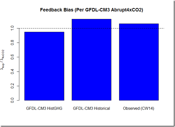
Finally, if one where to calculate the feedback bias relative to the abrupt4xCO2 scenario, we find the following ratios:

GFDL_CM3_Feedback_Bias

This essentially isolates the expected forcing “enhancement” bias, as it is baselined against the idealized 4xCO2 run.  In this case, the above ratios are 0.95 (histGHG),  1.13 (historical), and 1.06 (observed).  This suggests that if one used the historicalGHG runs to estimate ECS, there might be a slight overestimate relative to the CO2-only run, as GFDL-CM3 includes the inhomogenous ozone forcing in their histGHG runs.  Were one to trust the relative strength of zonal feedbacks in GFDL-CM3, it suggests about a 6% underestimate of ECS from energy balance methods over the instrumental period due to the inhomogenous aerosol forcings.  However, ideally one could use this method with a variety of GCMs to identify the expected bias among a wider array of models.

Moreover, if one were interested in the bias of “effective sensitivity” (EFS) relative to ECS, one would ideally get a longer run of GFDL-CM3 with a doubling (or quadrupling) of CO2, and see how the warming pattern ended up after it reached equilibrium.  Unfortunately, I am not aware of any such output currently available for this model. 

***Final note: in my calculations, I initially performed the analysis using land and ocean zonal feedbacks and temperatures separately, rather than combined into one.  For GFDL-CM3, this did not seem to make much difference, and I did not readily have available separately gridded land and ocean temperatures from observations.  However, I seem to recall that the response was substantially different between land and ocean in Armour et al (2013), so perhaps it a more wide-ranging survey of GCMs it would be better to separate these out again.

Does anybody else think this a promising method for leveraging historical observations in estimating the potential bias in energy balance estimates?

Code and Data

May 9, 2014

On forcing enhancement, efficacy, and Kummer and Dessler (2014)

Filed under: Uncategorized — troyca @ 10:11 pm

A paper by Kummer and Dessler (2014) [KD14] has recently been accepted by GRL, with the primary claim being that observational estimates of ECS over the 20th century can be reconciled with the higher ECS of CMIP5 models by accounting for the “forcing efficacy” mentioned in Shindell (2014):

Thus, an efficacy for aerosols and ozone of ≈1.33 would resolve the  fundamental disagreement between estimates of climate sensitivity based on the  20th-century observational record and those based on climate models, the paleoclimate record, and interannual variations.

However, I think there is some fundamental confusion with respect to how the forcing enhancement should be applied within KD14, which I will focus on specifically for this post (ignoring what I believe to be other issues in the actual energy balance calculations for the mean time).  While I have noted previously that the spatial warming pattern appears to indicate a value of “E” (the Shindell enhancement) near unity, I would submit that even if it was significantly greater than 1.0, it has been applied in a way within KD14 that likely substantially exaggerates its effect on 20th century ECS calculations.  Here are the issues that I see:

1. ECS calculations are unaffected by the effective heat capacity, whereas TCR calculations are not

First, let’s take a look at the Shindell (2014) definition for the forcing enhancement (which KD14 refers to as “forcing efficacy”), which is the ratio of the inhomogenous forcing TCR to that of the homogenous forcing TCR:

(Eq. 1)        

TCR is calculated by dividing the temperature change by the forcing, without consideration of the TOA energy imbalance at the time of the calculation (this is often normalized to transient change for a doubling of CO2 by multiplying by F_2xCO2 (~3.7 W/m^2), but I will leave it simply in the units of K/(W/m^2) for this post):

(Eq. 2)       

And if we consider the simple one box temperature response to an imposed forcing at time t, we have:

(Eq. 3)      

Where F is the imposed forcing change, lambda is the strength of radiative restoration (the increase in outgoing flux per unit of surface warming), and C is the effective heat capacity of the system.  As can be seen by working back from equation 3 to 1, TCR and hence E  will be affected by both the difference in C (the heat capacity) and lambda (radiative restoration) between the homogenous and inhomogeneous forcings.  On the other hand, the equilibrium response (t –> infinity) to a forcing does NOT depend on C, only lambda.

If we go back to the simple energy balance equation for the top of the atmosphere (TOA) , re-arranging eq. 1 in KD14 to solve for lambda (with N representing this net TOA imbalance), we have:

(Eq. 4)     

which can then be inverted and multiplied by F_2xCO2 to find the ECS in terms of a CO2 doubling.  What should be quite clear from this determination of ECS is that one can dampen the transient temperature response by increasing the value of C without it affecting the estimate of ECS.  After all, If the temperature response is heavily damped in the first 50 years for a forcing (due, for example, to the bulk of that forcing being concentrated in an area with deep oceans), then it is true that the value for T will be lower than it might be for a scenario with less ocean damping, but  the TOA imbalance (N) will be larger due to less radiative response (from lambda * T), thereby decreasing the quantity (F-N) by the same ratio , and yielding the same value for lambda.  On the other hand, it is clear why such ocean damping *would* affect the TCR, which does not take into account the TOA imbalance (N).

The problem should thus be obvious: the “enhancement” factor calculated by Shindell (2014) can be greatly affected by the difference in effective heat capacity of the hemispheres, but this in itself would not create any bias in the ECS calculations.  So KD14 should certainly not be using the forcing “enhancement” factor of Shindell as a proxy for the equilibrium forcing efficacy!  Note that much discussion regarding Shindell (2014) focused on how the greater land mass of the NH corresponds to a lower heat capacity, thus producing a greater transient response for an aerosol forcing located primarily in the NH.   But this intuition has nothing to do with a bias in the equilibrium response.

Rather, as I mentioned above, E is affected by both the effective heat capacity differential (C) and the increase in outgoing flux per unit increase in temperature (lambda), only the latter of which actually affects ECS.  So the more we find that E is a result of the differing heat capacity, the less room that leaves for lambda to have a substantial effect, and the less bias this would actually produce in the ECS estimates.  Furthermore, there seems to be less of the way in intuition of why a differing lambda would be responsible for a substantial portion of E, if this were the case.  Nevertheless, it IS possible that for a larger E, at least some portion of this would come from a differing radiative response strength from homogenous and inhomogenous forcings, but that leads to the second issue…

2. The Forcing Efficacy “correction” in the estimate is applied directly to the TOA imbalance resulting from the forcing, thereby overcompensating in transient estimates

Per KD14, we read that:

To test the impact of efficacy on the inferred λ and ECS in our calculations, we multiply the aerosol and ozone forcing time series by an efficacy factor in the calculation of the total forcing.

What Kummer and Dessler (2014) have done here is simply inflated the magnitude of the aerosol and ozone forcings beyond the best estimates, rather than actually accounting for the forcing “efficacy” that may result from differing lambdas.  In the event that the TOA imbalance has already reached equilibrium, there is no need for this distinction.  But in transient runs, using the KD14 method will bias the ECS high, because it is compensating for the differing TOA response in the numerator of Eq. 4 that has not yet fully manifested!

Consider an example, where lambda is 1.5 W/m^2/K for GHG (~2.5 K “true” ECS), but the “forcing efficacy” for aerosols is 1.5 and entirely comes from differing lambda, such that lambda for aerosols is 1.0 W/m^2/K.  Now suppose we perform our calculation early on in the transient run, such that only 50% of the equilibrium response to a given forcing of 2.0 W/m^2 GHG and –1.0 W/m^2 aerosols has been achieved.  This will yield T_GHG = 2.0 / 1.5 * 50% = 0.67 K, and T_aero = –1.0 / 1.0 * 50% = –0.5 K, for a net T of 0.17 K.  Using the KD14 method with Eq. 4, we would have an F = 2.0 W/m^2 – 1.5 * 1.0 W/m^2) = 0.5 W/m^2, an N of (2.0 W/m^2 – 1.0 W/m^2)  – [0.67 K * (1.5 W/m^2/K) + (-0.5 K) * (1.0 W/m^2/K) ]= .495 W/m^2, leading to a lambda of (0.5 – 0.495) / (0.17 K) = 0.03 W/m^2/K, corresponding to a sensitivity of > 100K!  This extreme example highlights the large bias that the KD14 method can produce when applied to transient runs.  Currently, if one takes the last decade net TOA imbalance to be ~ 0.6 W/m^2, and the forcing up to now to be ~ 2.0 W/m^2, this implies we are about 70% equilibrated…under these circumstances I would still expect a large bias from the KD14 application.

Anyhow, to illustrate the bias we would expect from the different methods of calculating ECS given an E of 1.5, I have written a script here.  Essentially, it treats the two hemispheres as separate one-box models, with the historic non-GHG anthropogenic forcings applied entirely to a more sensitive NH.  I have tried to match this to some degree so that the ending TOA imbalance is around 0.5 W/m^2 (and hence around 70% equilibrated), similar to that observed, but it is also possible that these models have oversimplified things.  Nevertheless, here are the results:

image

What this illustrates is much of the intuition we have gone over in these two sections.  From the blue line, we see that as we increase the attribution of the calculated E  to the heat capacity differential, there is very little bias introduced when calculating ECS using the “traditional” energy balance method (per #1 above, this is because there is less attributable to the difference in lambda) .  On the other hand,  since we introduce a case here where we are still far from equilibrium, the KD14 method creates an overestimate in all cases.

Summary

Overall, I am quite dubious about the KD14 results, for 3 reasons:

1) Based on the observed spatial warming, it seems unlikely that E is far from unity.

2) Even if E were greater than 1.0, only a fraction of that E applies to ECS estimates (the portion stemming from differential lambdas and NOT heat capacities), and

3) Even if the full E did apply, it appears KD14 has applied it incorrectly, introducing a large overestimate in the transient cases

The shame of it all is that this actually hints at an interesting underlying question, which is whether the spatial pattern of warming in the real world has created a radiative response substantially different from the response expected from a uniform GHG forcing.  It seems that if one were interested in what models say, however, it could be calculated much more directly – comparing the AMIP simulated radiative restoration strength to that of the historicalGHG from the same models would likely be the way to begin along this path.

May 1, 2014

Effective vs. Equilibrium Sensitivity: Uncertainty in projections resulting from the CMIP5 OHU efficacy range in a two-layer model

Filed under: Uncategorized — troyca @ 9:20 pm

A somewhat frequent topic that has come up here has been the difference between effective sensitivity and equilibrium sensitivity; that is, the extent to which the increase in outgoing radiative flux per unit increase in temperature may change over time.  Given the timescales involved, the relationship between “effective” sensitivity calculated over some transient time period (typically 100-200 years) and equilibrium sensitivity is nearly impossible to observe in the real world, so experiments so far have been primarily model-based, such as in Armour et al, 2013 and Rose et al., 2014.  The abstract of the latter study concludes with: “Results imply that…equilibrium climate sensitivity cannot be reliably estimated from transient observations.”  While certainly interesting from an academic perspective, I have found myself wondering whether this result is actually relevant to projection of future anthropogenic warming.  After all, if “effective” sensitivity (EFS), which is calculated on century timescales, significantly deviates from equilibrium sensitivity (ECS, which applies to millennial timescales), then it would seem to suggest that EFS should be the focus when determining policy / projections. 

One way to model this contrast in EFS vs. ECS is using a factor for “efficacy” (not “efficiency”, which is a separate concept) of ocean heat uptake (OHU), per Winton et al., 2010 and Held et al., 2010.  In Geoffroy et al., 2013 Part II (the first part of which I’ve been referencing for my two-layer model), the authors indicate that such a two-layer model with this efficacy factor is generally able to represent the global behavior of the CMIP5 AOGCMs:


and


Here C and C_0 represent the heat capacities of the atmosphere+ocean mixed layer and deeper ocean respectively, T and T_0 represent the temperature anomalies for those layers, gamma represents the heat transfer rate between those layers, epsilon represents the efficacy of ocean heat uptake, F represents the TOA forcing, and lambda represents the equilibrium radiative restoration strength. 

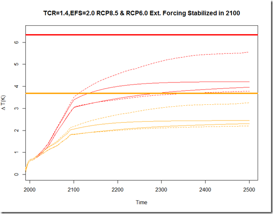
Anyhow, using this representation suites my purpose here, as I want to isolate the uncertainty in the RCP projections that might result exclusively from the uncertainty in this efficacy parameter.  Essentially, I want to answer this question: if we remove almost all uncertainty from the magnitude/efficacy of forcings, temperature observations, natural variability, and TOA imbalance, such that  we could constrain the TCR and EFS calculated from 1860-1879 to 2000-2009 to 1.4 K +/- 0.05 and 2.0 K +/- 0.05 respectively (similar to the most likely estimates of Otto et al. (2013)), what sources of uncertainty would remain for the respective RCP scenario projections?  In this two-layer model, there are three parameters that can be tuned if we assume ECS = EFS while constraining to the TCR=1.4 and EFS=2.0 calculations mentioned previously: C, C_0, and gamma.  As there is no unique solution set, I only sample from the range of values calculated in Geoffroy et al., 2013 for the CMIP5 AOGCMs for each of the parameters, which still yields a large ensemble of models (that is, parameter combinations).  Now, if we don’t assume ECS = EFS, we can vary two more parameters: efficacy and lambda.  Once again I constrain efficacy to be within the range of values calculated by  Geoffroy et al., 2013 for that set of AOGCMs, while allowing lambda to be a “free” parameter.  This obviously gives a larger ensemble of models than when only allowing the ocean parameters to be modified. 

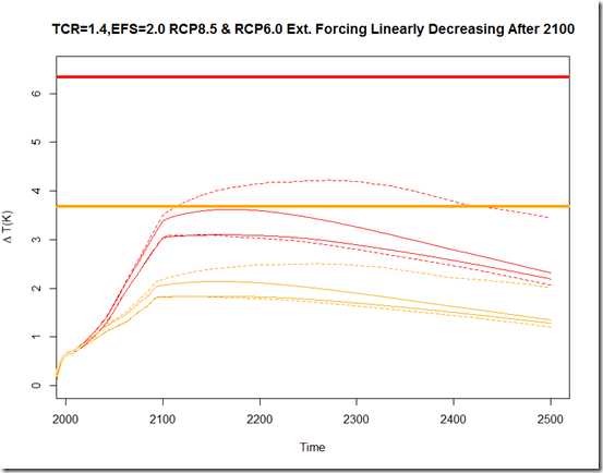
The next step is to run these models with the adjusted RCP forcings calculated in Forster et al., 2013.  I have extended these forcing beyond 2100 using two simple scenarios: the first is to maintain the forcing in 2100 through 2500, while the second linearly decreases the forcing from 2100 to 2500 so that the value in 2500 is half (relative to pre-industrial) of what it was in 2100.  From here, if we compare the 2.5%-97.5% interval from the only-ocean-modified-parameters ensemble (solid lines) with that of the efficacy-modified ensemble (dashed lines), we can see the practical difference in EFS vs. ECS in these future projections.  These first two figures show the aforementioned scenarios for RCP8.5 (red) and RCP6.0 (orange), with the thick lines representing the equilibrium temperature response to the scenario forcing if ECS=3.0 (noting that the dashed 97.5% upper-limit essentially represents a model with an ECS=3.0 and EFS=2.0).

rcp_high_emit_linear_stabilized

rcp_high_emit_linear_decreasing

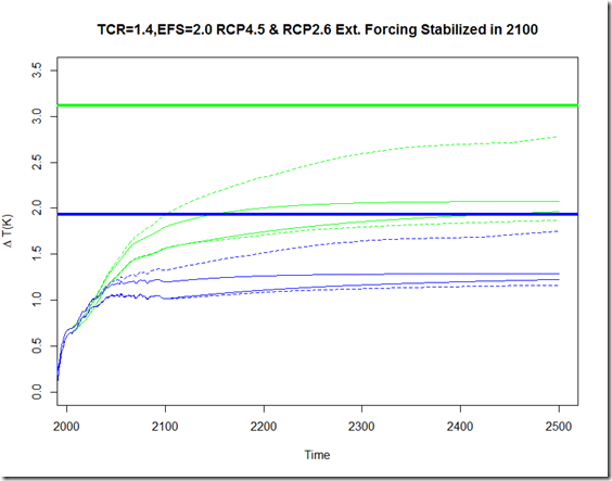
And these next two figures show the same thing for RCP4.5 (green) and RCP2.6 (blue):

rcp_low_emit_linear_stabilized


rcp_low_emit_linear_decreasing

As can be seen, the uncertainty from the efficacy of OHU does not really manifest itself prior to 2100 in the projections.  Beyond that, the high-end uncertainty increases for the varying-efficacy ensemble relative to the fixed efficacy model, although the behavior largely depends on the behavior of the forcings after 2100.  In the event that these forcings are fixed for the subsequent 400 years, the high-end efficacy separates itself from the effective sensitivity path and continues marching towards the equilibrium temperature change.  In the event that the forcings begin to decrease after 2100, even the high-end efficacy never comes particularly close to its equilibrium change.

I should note that not too much should be made about the asymmetric nature of the varying-efficacy uncertainty bounds.  This is a consequence of simply using a uniform sampling of efficacy from the range of CMIP5 models (0.8 – 1.8), and obviously since an efficacy > 1.0 implies an ECS > EFS, we are grabbing higher-up in the efficacy range.  Whether these CMIP5 AOGCMs represent a reasonable range for the efficacy is a reasonable question, but I’m not sure it has an easy answer.    

Script is available here

March 15, 2014

Does the Shindell (2014) apparent TCR estimate bias apply to the real world?

Filed under: Uncategorized — troyca @ 9:35 am

There has been some considerable discussion of Shindell (2014) and the suggestion that usual estimates of TCR (which assume roughly equal efficacies for different forcings), such as Otto et al, (2013), might be underestimating TCR with the traditional method.  A few example discussing Shindell (2014) are at Skeptical Science, And Then There’s Physics, and Climate Audit.  SkS’s Dana went so far as to say the paper “demolishes” Lewis and Crok’s report at James Annan’s blog, but JA responds quite skeptically of the Shindell (2014) results.

On the face of it, the argument is fairly simple and intuitive (so buyer beware!): since the cooling effect of aerosols generally occur in the Northern Hemisphere where there is greater land mass and thus lower effective heat capacity, these forcings will disproportionally affect the global temperature relative to the forcing of well-mixed greenhouse gases, which acts globally.  Since Watt per Watt these cooling forcings will give you more bang for your buck, an estimate of TCR using only the globally averaged forcing and global temperature could be biased low.  Shindell (2014) therefore tries to find the average “enhancement” of aerosol+O3 forcings, E, through GCMs, and uses the following to calculate TCR from global quantities:

TCR = F_2xCO2 x (dT_obs / (F_ghg + E x (F_aerosols + F_Ozone + F_LU)))

However, there are reasons to be skeptical of this result as well.  For one, there *have* been studies that specifically looked at the rate of warming and certainly don’t assume homogenous forcings, such as Gillett et al (2012), which find low TCR estimates consistent with Otto et al., (2013).  Furthermore, Shindell (2014) does not seem to consider the ratio of observed warming in the NH vs. SH. ..using Cowtan and Way (2013) with HadCRUT4 kriging, from the base period (1860-1879) through the end of the historical simulation time period (1996-2005), the ratio of NH warming to SH warming is 1.48.  Obviously, if there was a large cooling effect from aerosols concentrated primarily in the NH (due to a large enhancement of the aerosol effect), we would expect to see more warming in the SH than the NH!  Third, there did not seem to be any tests run on the actual historical simulations from models, which would tell us how well the Shindell (2014) method performs relative to the “simple” E=1.0 method (e.g. Otto et al).  These last tests should be easy to pass, since the value of “E” would be calculated from the same model that the tests are run on (unlike the real world, where we don’t know the “true” value of E).

The first table simply shows the forcings and temperature changes using the same models as S14, as much of this information is available in the supplement.  These tests will be based on the difference between the base period (1860-1879) and the end of the historical simulation (1996-2005) using the historical runs.

TABLE 1. Temperature + Forcing from historical simulations and Aero/O3 Enhancement (from Shindell 2014)

Model

ΔT

ΔF_WMGHG

ΔF_Aero_O3_LU

ΔF_2xCO2

E

IPSL-CM5-LR

1.15

2.40

-0.45

3.20

2.43

CanESM2

0.94

2.40

-0.69

3.70

1.18

GFDL-CM3

0.49

2.49

-1.12

2.99

1.57

CSIRO-MK-3.6.0

0.58

2.15

-1.13

3.10

1.18

HadGEM2-ES

0.53

2.27

-1.08

3.50

1.48

MRI,NOR,MIROC AVG

0.56

2.05

-0.83

3.65

1.40

One thing that has been nagging me about this is that natural forcings are not included in the TCR equation above.  I am not sure if the slightly positive solar influence is balanced out by the slightly negative volcanic influence in models, or what, but S14 does not include estimates of these natural forcings in the models so I have not included them in the tests either. And here are the results of the actual tests using the above numbers: 

TABLE 2. Estimate of TCR using Simple (E=1.0) estimate vs. Shindell (2014) methods, along with NH/SH warming ratios

Model

Simple Estimate (K)

Shindell Estimate(K)

TCR Actual (K)

Error_Simple

Error_Shindell

NH/SH Hist

NH/SH HistGHG

IPSL-CM5-LR

1.88

2.79

2.00

-6%

40%

1.49

1.62

CanESM2

2.03

2.19

2.40

-16%

-9%

0.96

1.28

GFDL-CM3

1.07

1.98

2.00

-47%

-1%

0.84

1.90

CSIRO-MK-3.6.0

1.75

2.19

1.50

17%

46%

1.00

1.15

HadGEM2-ES

1.56

2.75

2.10

-26%

31%

1.17

1.70

MRI,NOR,MIROC

1.67

2.28

1.70

-2%

34%

1.58

1.60

Observed (CW13)


1.48


Assuming I have not messed something up here, these results appear to be very concerning for Shindell (2014).  For example, IPSL-CM5-LR, the model from S14 with the largest “enhancement” at E=2.43, would be expected to yield a major underestimate of TCR using the simple method.  Instead, the simple estimate only underestimates TCR by 6%, whereas applying the S14 “correction” makes things far worse, yielding a 40% overestimate of TCR!  In fact, in 4 of the 6 models, the Shindell method overestimates the TCR by > 30%.  On the other hand, the “simple” method only underestimates TCR by > 30% in 1 of the 6 cases.  

Perhaps even more concerning, however, is the specific model ensembles for which the Shindell (2014) method largely overestimates the TCR.  Given the observed NH/SH warming ratio of 1.48, the two models that are most realistic in this regard are IPSL-CM5-LR (1.49) and the average of MRI, NOR, and MIROC (1.58).   Since the argument from Shindell (2014) essentially hinges on the NH being disproportionately cooled by aerosols relative to the SH, these are the most directly relevant.  And yet, using the “simple” method in these cases produces underestimates of 6% and 2%, which would hardly change the results of a paper like Otto et al, 2013.  On the other hand, the Shindell (2014) “correction” causes overestimates of 40% and 34%  (e.g. a shift from a 1.3K “most likely” value from Otto to the 1.7K reported by S14).  If we look at the model that the “simple” method largely underestimates, GFDL-CM3, we see that the 0.84 NH/SH in that model is the farthest away from the one we’ve observed in the real world, suggesting it is likely the least relevant. 

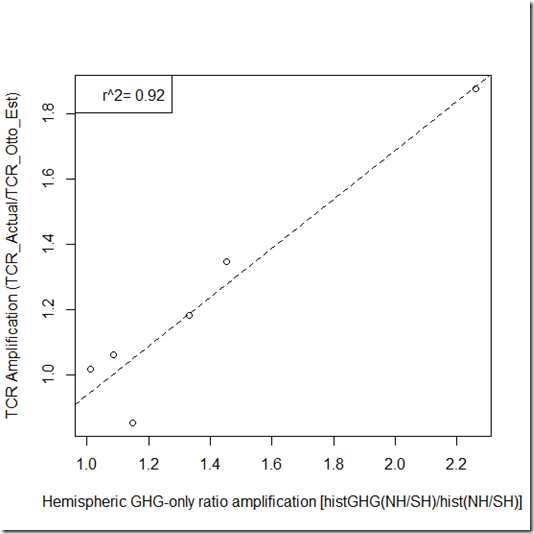
In fact, I would argue that the amplification of the NH/SH ratio in the historicalGHG simulation relative to the historical simulation for a model could be used to better estimate the TCR “bias” calculated using that model.  This is because the difference in the NH/SH ratio in the historicalGHG simulation and that of the historical simulation implicitly combines the actual aerosol forcing and the “enhancement” of this forcing (rather than trying to estimate these highly uncertain values separately), which is even more directly relevant to the degree of TCR bias.  Indeed, if we look here, there appears to be excellent correlation:


image


Impressive, eh?   Now, I will mention that I believe things to be less pretty than the r^2=0.92 value shown above.  This is primarily because the 3 models bundled in Shindell et al (2014) actually have very different rates of global warming, as well as the NH/SH ratios, so I’m not sure it makes sense to bundle them, but have done so here for consistency with S14. 

One problem with using my method here and applying it to the“real-world”  is that we don’t know what the NH/SH warming ratio would be for the real world in the GHG-only scenario.  However, given the high value of 1.48 observed for the real-world “all-forcing” case, I suspect that the difference between this ratio and the GHG-only scenario can’t be that large, unless models have seriously underestimated the historicalGHG warming ratios.  Moreover, I would argue that the value is likely to be better constrained from models than the value of E, which depends on the much more uncertain aerosol properties.   Regardless, the average model warming ratio for NH/SH for the historicalGHG simulations in the above models is 1.54.  If you plug in the observed value of 1.48 for the “historical” observed NH/SH ratio in the real world, and use the linear regression from above, the estimated TCR bias amplification factor is 0.96.  This would suggest using the “simple” method slightly overestimates TCR, but by an extremely small fraction. 

Conclusion

While Shindell (2014) uses several GCM results to argue that traditional methods to calculate TCR lead to an underestimate, testing these methods against the outputs of those same GCMs seems to suggest the “simple” (E=1.0) methods perform better than the S14 “corrected” method.  Furthermore, when we consider the actual observed NH/SH warming ratio, it also seems to suggest that the TCR bias in the traditional/simple method is either very small or non-existent. 

Data and code.

March 11, 2014

How sensitive are the Otto et al. TCR and ECS estimates to the temperature and ocean heat datasets?

Filed under: Uncategorized — troyca @ 10:59 pm

There seems to have been some interest in the sensitivity of Otto et al. (2013) lately.  For instance, see Piers Forster’s comments about HadCRUT4 in Otto, or Trenberth and Fasullo (2014), which notes that using ORAS-4 for the OHC dataset raises the estimate of ECS from 2.0 to 2.5 K.   Anyhow, I ran a few of the tests, and thought I would share the results. 

Otto et al (2013) uses five different intervals over which the differences of temperature, forcing, and TOA imbalance (for the ECS estimate) are calculated: 1) 2000s – Base, 2) 1990s – Base, 3) 1980s – Base, 4) 1970s – Base, and 5) the 40 year interval from 1970-2009.  The base period used is 1860-1879.  Here are the results when using the BEST or Cowtan and Way (2013) global temperature datasets (which infill under-sampled regions to get more global coverage)  to calculate TCR alongside HadCRUT4:


ΔF (W/m^2)

HadCRUT4 ΔT (K)

HadCRUT4 TCR (K)

CW13 ΔT (K)

CW13 TCR (K)

BEST ΔT (K)

BEST TCR (K)

2000s-Base

1.94

0.75

1.33

0.81

1.44

0.81

1.44

1990s-Base

1.25

0.57

1.57

0.6

1.65

0.6

1.65

1980s-Base

0.99

0.39

1.36

0.43

1.49

0.44

1.53

1970s-Base

0.75

0.22

1.01

0.26

1.19

0.27

1.24

2009-1970

1.28

0.53

1.42

0.56

1.51

0.54

1.45

In most situations, it appears that the difference is relatively small, adding ~0.1K of TCR when using either Cowtan and Way (2013) or BEST global temperatures.    
   
For ECS, I used Cowtan and Way (2013) for the temperature dataset and three different ocean heat content datasets: 1) Lyman and Johnson (2014), 2)  ORAS-4, the reanalysis product introduced in Balmaseda et al. (2013), and 3) Levitus et al (2012).  For #1 and #2, I digitized the values from their respective papers.  Since the calculation of ECS is slightly more complicated, I have included additional steps along the way.  OHU represents the rate of ocean heat uptake as calculated over the period from the observed ocean heat content,  and ΔQ represents the change in TOA imbalance over the interval (I assume 90% of the TOA imbalance goes into the ocean, and per Otto et al that the imbalance of the base period was 0.08 W/m^2).  I also include a “most recent” period calculation, which occurs if we measure the OHC after the bulk of the ARGO deployment took place.  For LJ14 they present this value from 2004-2011.  For L12, they don’t present annual estimates until 2005, so I’ve used 2005-2013.  For B13, I simply used 2004-2010.  Here are the results:


ΔF (W/m^2)

CW13 ΔT (K)

LJ14 OHU (W/m^2)

LJ14 ΔQ (W/m^2)

LJ14 ECS (K)

B13 OHU (W/m^2)

B13 ΔQ (W/m^2)

B13 ECS(K)

L12 OHU (W/m^2)

L12 ΔQ (W/m^2)

L12 ECS (K)

2000s-Base

1.94

0.81

0.50

0.48

1.90

0.85

0.86

2.59

0.48

0.45

1.87

1990s-Base

1.25

0.60

0.25

0.20

1.96

-0.22

-0.32

1.31

0.25

0.20

1.96

1980s-Base

0.99

0.43

-0.26

-0.37

1.09

0.49

0.46

2.81

0.13

0.06

1.60

1970s-Base

0.75

0.26

0.32

0.28

1.89

0.16

0.10

1.37

0.49

0.46

3.13

2009-1970

1.28

0.56


0.20

1.78


0.77

3.75


-0.01

1.49

Post_ARGO(2004 or 2005)-Base

1.94

0.85

0.29

0.24

1.72

0.51

0.49

2.01

0.54

0.52

2.06

As you can see, the bulk of the estimates still seem to suggest an ECS < 2K, in line with the Otto et al (2013) calculations.  For LJ14, the results are actually pretty tightly constrained (apart from the “low-ball” 1980s estimate) between 1.7 and 2.0 K.  Using ORAS-4 (B13) does increase the ECS estimate when using the 2000s only, but it also largely decreases when using the 1990s or 1970s.  When using only post-ARGO data, it is pretty much in line with the others, suggesting an ECS ~ 2K.  L12 is also fairly tightly constrained, apart from the “highball” estimate of the 1970s.  Overall,using ORAS-4 produces the largest error margins and interval-specific sensitivity. However, it is worth noting that using the post-ARGO OHC data seems to largely remove the dependence on which OHC dataset is chosen, producing best estimates between 1.7 and 2.1 for ECS. 

Data for this post available here.

February 28, 2014

Initial thoughts on the Schmidt et al. commentary in Nature

Filed under: Uncategorized — troyca @ 7:20 pm

Thanks to commenter Gpiton, who on my last post about attributing the pause, alerted me to the commentary by Schmidt et al (2014) in Nature (hereafter SST14).  In the commentary, the authors attempt to see how the properties of the CMIP5 ensemble and mean might change if updated forcings were used (by running a simpler model), and find that the results are closer to the observed temperatures (thus primarily attributing the temperature trend discrepancy to incorrect forcings).  Overall, I don’t think there is anything wrong with the general approach, as I did something very similar in my last post.  However, I do think that some of the assumptions about the cooler forcings in the "correction" are more favorable to the models than others might choose, and a conclusion could easily be misinterpreted.  This is my list of comments that, were I a reviewer, I would submit:

Comment #1: The sentence

We see no indication, however, that transient climate response is systematically overestimated in the CMIP5 climate models as has been speculated, or that decadal variability across the ensemble of models is systematically underestimated, although at least some individual models probably fall short in this respect.

is vague enough to perhaps be technically true while at the same time giving the (incorrect, IMO) impression they have found that models are correctly simulating TCR or decadal variability.  It may be technically true in that they find "no indication" of bias in TCR or internal variability, due to the residual “prediction uncertainty”, but this is one of those "absence of evidence is not evidence of absence" scenarios, where even if the models WERE biased high in their TCR there would be no indication by this definition.  By the description in the commentary,  the adjustments only remove about 60-65% of the discrepancy.  The rest of the discrepancy may be related to non-ENSO noise, but it also may be related to TCR bias, and would be what we expect to see if , for example, the "true" TCR was 1.3K (as in Otto et al., 2013) vs. the CMIP5 mean of 1.8K.  Obviously, the reference to Otto et al., (2013) might be mistaken by some to suggest an answer/refutation to that study (which used a longer period to diagnose TCR in order to reduce the "noise"), but clearly this would be wrong.  Had I been a reviewer, I would have suggested changing the wording: "The residual discrepancy may be consistent with an overestimate of the transient climate response in CMIP5 models [Otto et al., 2013] or an underestimate of decadal variability, but it is also consistent with internal noise unrelated to ENSO, and we thus cannot neither rule out nor confirm any of the explanations in this analysis."  Certainly has a different feel, but it essentially communicates the same information, and is much less likely to be misinterpreted by the reader.

Comment #2: Regarding the overall picture of updated forcings, it is worth pointing out that IPCC AR5 Chapter 9  [Box 9.2, p 770] describes a largely different opinion (ERF = ”effective radiative forcing”)

For the periods 1984–1998 and 1951–2011, the CMIP5 ensemble-mean ERF trend deviates from the AR5 best-estimate ERF trend
by only 0.01 W m–2 per decade (Box 9.2 Figure 1e, f). After 1998, however, some contributions to a decreasing ERF trend are missing
in the CMIP5 models, such as the increasing stratospheric aerosol loading after 2000 and the unusually low solar minimum in 2009.
Nonetheless, over 1998–2011 the CMIP5 ensemble-mean ERF trend is lower than the AR5 best-estimate ERF trend by 0.03 W m–2 per
decade (Box 9.2 Figure 1d). Furthermore, global mean AOD in the CMIP5 models shows little trend over 1998–2012, similar to the
observations (Figure 9.29). Although the forcing uncertainties are substantial, there are no apparent incorrect or missing global mean
forcings in the CMIP5 models over the last 15 years that could explain the model–observations difference during the warming hiatus.

(My emphasis).  Essentially, the authors of this chapter find a discrepancy of 1.5 * 0.03 = 0.045 W/m^2 over the hiatus, whereas SST14 use a discrepancy of around 0.3 W/m^2, which is nearly 7 times larger!  And there does not appear to have been new revelations about these forcings since the contributions to the report were locked down – the report references the "increasing stratospheric aerosol loading after 2000" and "unusually low solar minimum in 2009" mentioned in the  commentary.  Regarding the anthropogenic aerosols, both the Shindell et al, (2013) and  Bellouin et al., (2011) papers referenced by SST14 for the nitrate and indirect aerosol estimates are also referenced in that AR5 chapter, and Shindell was a contributing author to the chapter.  This is not to say that the IPCC is necessarily right in this matter, but it does suggest that not everyone agrees with the magnitude of the forcing difference used in SST14.

Comment #3:  Regarding the solar forcing update, per box 1, SST14 note: "We multiplied the difference in total solar irradiance forcing by an estimated factor of 2, based on a preliminary analysis of solar-only transient simulations, to account for the increased response over a basic energy balance calculation when whole-atmosphere chemistry mechanisms are included."

I would certainly want to see more justification for doubling the solar forcing discrepancy (this choice alone accounts for about 15% of the 1998-2012 forcing discrepancy used)!  If I understand correctly, they are saying that they found that the transient response to the solar forcing is approximately double the response to other forcings in their preliminary analysis.  But this higher sensitivity to a solar forcing would seem to be an interesting result in its own right, and I would want to know more about this analysis, and what simulations were used – was this observed in one, some, most, or all of the CMIP5 models?  After all, if adjusting the CMIP5 model *mean*, it would be important to know that this was a general property shared across most of the CMIP5 models.

Comment #4: For anthropogenic tropospheric aerosols, two adjustments are made.  One for the nitrate aerosol forcing, and the second for the aerosol indirect effect.  SST14 notes that only two models include the nitrate aerosol forcing, whereas half contain the aerosol indirect effect, and so the ensemble and mean are adjusted for these.  But it is not clear to me if the individual runs for each of the CMIP5 models are adjusted (and thereby no adjustments are made to runs from models that include the effect), and the mean recalculated, or if simply the mean is adjusted.  The line "…if the ensemble mean were adjusted using results from a simple impulse-response model with our updated information on external drivers" makes me think the latter.  But if it is this latter case, clearly this is incorrect – if half of the models already include the effect, you would be overcorrecting by a factor of 2 if you adjusted the mean by this full amount (perhaps the -0.06 is halved before the adjustment is actually made, but it is not specified).

Comment #5: Regarding the indirect aerosol forcing, Belloin et al., (2011) is used as the reference, which uses the HadGEM2-ES model.  It is worth noting the caveats:

The first indirect forcing in HadGEM2‐ES, which can be diagnosed to the first order as the difference between total and direct forcing [Jones et al., 2001] might
overestimate that effect by considering aerosols as externally mixed, whereas aerosols are internally mixed to some extent.  By comparing with satellite retrievals, Quaas et al. [2009] suggest that HadGEM2 is among the climate models that overestimate the increase in cloud droplet number concentration  with aerosol optical depth and would therefore simulate too strong a first indirect effect.

Moreover, I am not quite sure the origin of the -0.06 W/m^2.  Belloin et al., (2011) suggest an indirect effect from nitrates that is ~40% the strength of the direct effect.  So if only nitrate aerosols increased over the post-2000 period, I would expect an indirect effect of ~ -0.01 W/m^2.  It seems to me that this must include the much-larger effect of sulfate aerosols, which leads me to my next comment…

Comment #6: Sulfate Aerosols.  Currently, sulfate aerosols constitute a much larger portion of the aerosol forcing than do other species (nitrates in particular).  I presume that for #5, the indirect aerosol forcing of that magnitude would need to result from an increase in sulfur dioxide emissions.  But as per the reference of Klimont et al., (2013) in my last post, global sulfur dioxide emissions have been on the decline since 1990, and since 2005 (when the CMIP5 RCP forcings start) the Chinese emissions have been on the decline as well (only India continues to increase).  Rather than the lack of indirect forcing artificially warming the models relative to observations, it seems like it has been creating a *cooling* bias over this period, if you use the simple relationship between emissions and forcing as in Smith and Bond (2014).  In fact, since 2005 (according to Klimont et al., 2013 again), sulfur dioxide emissions have declined faster than in 3 of the 4 RCP scenarios.  It seems likely to me that the decline in sulfur dioxide emissions over this period (and it’s corresponding indirect effect) would more than counteract the tiny bias from the NO2 emissions. 

Conclusion:

Having just done a similar analysis, I thought it important to put the Schmidt et al. (2014) Nature commentary in context.  There is enough uncertainty around the actual forcing progression during the "hiatus" to find a set of values that attribute most of the CMIP5 modeled / observed temperatures to forcing differences.  However, the values chosen by SST14 do seem to represent the high end of this forcing discrepancy, and it appears that most of authors of AR5 chapter 9 believe the forcing discrepancy to be much more muted.  Moreover, the SST14 commentary should not be taken to be a response to longer period, more direct estimates of TCR, such as that of Otto et al., (2013).  Specifically, the TCR bias found in that study would be perfectly consistent with the remaining discrepancy and uncertainty present between the CMIP5 models and observations.    

February 21, 2014

Breaking down the discrepancy between modeled and observed temperatures during the “hiatus”

Filed under: Uncategorized — troyca @ 9:35 pm


Introduction

There are many factors that have been proposed to explain the discrepancy between observed surface air temperatures and model projections during the hiatus/pause/slowdown. One slightly humorous result is that many of the explanations used by the “Anything but CO2” (ABC) group – which argues that previous warming is caused by anything (such as solar activity, the PDO, or errors in observed temperatures) besides CO2 – are now used by the “Anything but Sensitivity” (ABS) group, which seems to argue that the difference between modeled and actual temperatures may be due to anything besides oversensitivity in CMIP5 models. And while many of these explanations likely have merit, I have not yet seen somebody try to quantify all of the various contributions together. In this post I attempt (perhaps too ambitiously) to quantify likely contributions from coverage bias in observed temperatures, El Nino Southern Oscillation (ENSO), post-2005 forcing discrepancies (volcanic, solar, anthropogenic aerosols and CO2), the Pacific Decadal Oscillation (PDO), and finally the implications for transient climate sensitivity.

Since the start of the “hiatus” is not well defined, I will consider 4 different start years, all ending in 2013. 1998 is often used because of the large El Nino that year, which minimizes the magnitude of the trend starting in that year.  On the other hand, the start of the 21st century is sometimes considered as well. Moreover, I will use HadCRUTv4 as the temperature record (since this is the more cited to represent the hiatus), which will show a larger discrepancy at the beginning than GISS, but will also show a larger influence from the coverage bias. The general approach here is to consider that IF the CMIP5 multi-model mean (for RCP4.5) is unbiased, what percentage of the discrepancy can we attribute to the various factors? Only at the end do we look into how the model sensitivity may need to be “adjusted”. Note that each of the steps below are cumulative, building off of previous adjustments. Given that, here is the discrepancy we start with:

Start year

HadCRUT4 (K/Century)

RCP4.5 MMM (K/Century)

1998

0.44

2.27

1999

0.75

2.16

2000

0.44

2.01

2001

-0.08

1.92


Code and Data

My script and data for this post can all be downloaded in the zip package here. Regarding the source of all data:

· Source of “raw” temperature data is HadCRUTv4

· Coverage-bias adjusted temperature data is from Cowtan and Way (2013) hybrid with UAH

· CMIP5 multi-model mean for RCP4.5 comes from Climate Explorer

· Multivariate ENSO index (MEI) comes from NOAA by way of Climate Explorer

· Total Solar Irradiance (TSI) reconstruction comes from SORCE

· Stratospheric Aerosol Optical Thickness comes from Sato et al., (1993) by way of GISS

· CMIP5 multi-model mean for natural only comes from my previous survey

· PDO index comes from the JISAO at the University of Washington by way of Climate Explorer.


Step 1: Coverage Bias

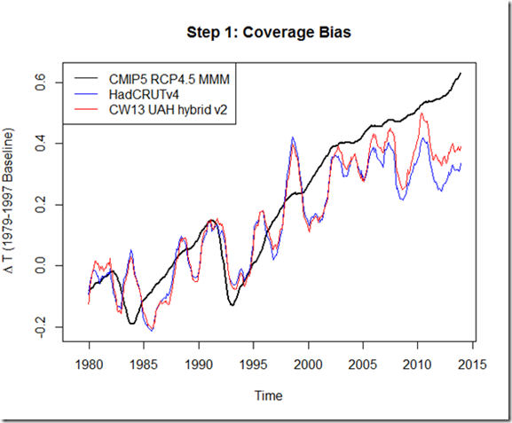
For the first step, we represent the contribution from coverage bias using the results from Cowtan and Way (2013). This is one of two options, with the other being to mask the output from models and compare it to HadCRUT4. The drawback of using CW13 is that we are potentially introducing spurious warming by extrapolating temperatures over the Arctic. The drawback of masking, however, is that if indeed the Arctic is warming faster in reality than it is in the multi-model-mean, then we are missing that contribution. Ultimately, I chose to use CW13 in this post because it is a bit easier, and because it likely represents an upper bound on the “coverage bias” contribution. I may examine the implications of using masked output in a future post.

image

The above graph is baselined over 1979-1997 (prior to the start of the hiatus), which highlights the discrepancy that occurs during the hiatus.

Start year

S1: HadCRUT4 Coverage Adj (CW13, K/Century)

RCP4.5 MMM (K/Century)

1998

1.10

2.27

1999

1.38

2.16

2000

1.05

2.01

2001

0.54

1.92

Step 2: ENSO Adjustment

The ENSO adjustment here is simply done using multiple linear regressions, similar to Lean and Rind (2008) or Foster and Rahmstorf (2011), except using the exponential decay fit for other forcings, as described here.  While I have noted several problems with the LR08 and FR11 approach with respect to solar and volcanic attribution, which I mention in the next step, I also found that ENSO variations are high enough frequency so as to be generally unaffected by other limitations in the structural fit of the regression model.

image


Step 3: Volcanic and Solar Forcing Updates for Multi-Model-Mean

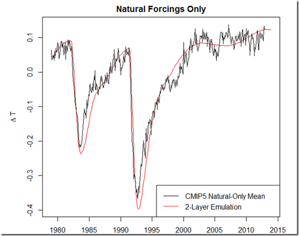
The next step in this process is a bit more challenging. We want to see to what degree updated solar and volcanic forcings would have decreased the multi-model mean trend over the hiatus period, but it is quite a task to have all the groups re-run their CMIP5 models with these updated forcings. Moreover, as I mentioned above and in previous posts (and my discussion paper), simply using linear regressions does not adequately capture the influence of solar and volcanic forcings. Instead, here I use a two-layer model (from Geoffrey et al., 2013) to serve as an emulator for the multi-model mean, fitting it to the mean of those natural-only forcing runs over the period. This is a sample of the “best fit”, which seems to adequately capture the fast response at least, even if it may be unable to capture the response over longer periods (but we only care about the updates from 2005-2013):

image


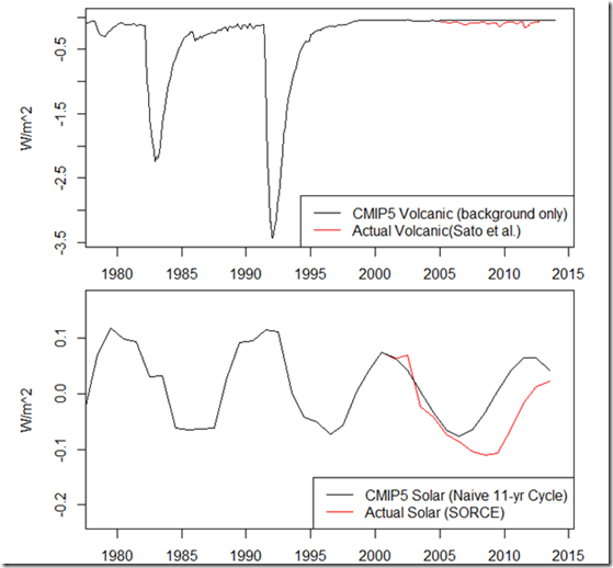
And here are the updates to the solar and volcanic forcings (updates in red). For the volcanic forcing, we have CMIP5 volcanic aerosols returning to background levels after 2005. For the solar forcing, we have CMIP5 using a naïve, recurring 11-year solar cycle, as shown here, after 2005.

image

The multi-model mean is then “adjusted” by the difference between our emulated volcanic and solar temperatures from the CMIP5 forcings and the observed forcings. The result is seen below:

image

Over the hiatus period, the effect of the updated solar and volcanic forcings reduces the multi-model mean trend by between 13% and 20%, depending on the start year.


Updated anthropogenic forcings?

With regards to the question of how updated greenhouse gas and aerosols forcings may have contributed to the discrepancy over the hiatus period, it is not easy to get an exact number, but based on evidence of concentrations and emissions that I’ve seen, there does not seem to be a significant deviation between the RCP4.5 scenario from 2005-2013 and what we’ve observed. This is unsurprising, as the projected trajectories for all of the RCP scenarios (2.6, 4.5, 6.0, 8.5) don’t substantially deviate until after this period.

For instance, the RCP4.5 scenario assumes the CO2 concentration goes from 376.8 ppm in 2004 to 395.6 ppm in 2013. Meanwhile, the measured annual CO2 concentration has gone from 377.5 ppm in 2004 to 396.5 ppm in 2013. By my back-of-the-envelopment calculation, this means we have actually experienced an increase in forcing of 0.002 W/m^2 more than in the RCP4.5 scenario, which is a magnitude away from being relevant here.

For aerosols, Murphy (2013) suggests little change in forcing from 2000-2012, the bulk of the hiatus period examined. Klimont et al (2013) find a reduction in global (and Chinese) sulfur dioxide emissions since 2005, compared to the steady emission used in RCP4.5 from 2005-2013, meaning that updating this forcing would actually increase the discrepancy between the MMM and observed temperatures. However, it seems safer to simply assume that mismatches between projected and actual greenhouse gas and aerosol emissions have contributed a likely maximum of 0% to the observed discrepancy over the hiatus, and it is quite possible that they have contributed a negative amount (that is, using the observed forcing would increase the discrepancy).


Step 4 & 5: PDO Influence and TCR Adjustment

Trying to tease out the “natural variability” influence on the hiatus is quite challenging. However, most work seems to point to the variability in the Pacific: Trenberth and Fasullo (2013) suggest the switch to the negative phase of the PDO is responsible, causing changing surface wind patterns and sequestering more heat in the deep ocean. Matthew England presents a similar argument, tying in his recent study to that of Kosaka and Xie (2013) over at Real Climate.

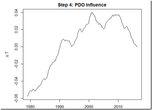
In general, the idea is that the phase of the PDO affects the rate of surface warming. If we assume that the PDO index properly captures the state of the PDO, and that the rate of warming is proportional to the PDO index (after some lag), we should be able to integrate the PDO index to capture the form of the influence on global temperatures. Unfortunately, because of the low frequency of this oscillation, significant aliasing may occur between the PDO and anthropogenic component if we regress this form directly against observed temperatures.

There are thus two approaches I took here. First, we can regress the remaining difference between the MMM adjusted for updated forcings and the ENSO-adjusted CW13, which should indicate how much of this residual discrepancy can be explained by the PDO. In this test, the result of the regression was insignificant – the coefficient was in the “wrong” direction (implying that the negative phase produced warming), and R^2=0.04. This is because, as Trenberth et al. (2013) note, the positive phase was in full force from 1975-1998, contributing to surface warming. But the MMM matches too well the rate of observed surface warming from 1979-1998, leaving no room for the natural contribution from the PDO.

To me, it seems that if you are going to leave room for the PDO to explain a portion of the recent hiatus, it means that models probably overestimated the anthropogenic component of the warming during that previous positive phase of the PDO. Thus, for my second approach, I again use the ENSO-adjusted CW13 as my dependent variable in the regression, but in addition to using the integrated PDOI as one explanatory variable, I include the adjusted MMM temperatures as a second variable. This will thus find the best “scaling” of the MMM temperature along with the coefficient for the PDO.

After using this method, we indeed find the “correct” direction for the influence of the PDO:

image

According to this regression, the warm phase of the PDO contributed about 0.1 K to the warming from 1979-2000, or about 1/3 of the warming over that period. Since shifting to the cool phase at the turn of the 21st century, it has contributed about 0.04 K cooling to the “hiatus”. This suggests a somewhat smaller influence than England et al. (2014) finds.

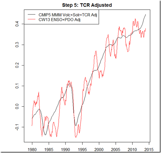
For the MMM coefficient, we get a value of 0.73. This would imply that the transient climate sensitivity is biased 37% too high in the multi-model mean. Since the average transient climate sensitivity for CMIP5 is 1.8 K, this coefficient suggests that the TCR should be “adjusted” to 1.3 K. This value corresponds to those found in other observationally-based estimates, most notably Otto et al. (2013).

When we put everything together, and perform the “TCR Adjustment” to the CMIP5 multi-model-mean as well, we get the following result:

image


Conclusion

Using the above methodology, the table below shows the estimated contribution by each factor to the modeled vs. observational temperature discrepancy during the hiatus (note that these rows don’t necessarily add up to 100% since the end result is not a perfect match):

Start Year

Step1: Coverage Bias

Step2: ENSO

Step3: Volc+Solar Forcings

Step4: PDO (surface winds & ocean uptake)

Step5: TCR Bias

1998

36%

10%

17%

2%

28%

1999

45%

0%

23%

6%

35%

2000

39%

9%

23%

7%

28%

2001

31%

16%

20%

5%

21%

According to this method, the coverage bias is responsible for the greatest discrepancy over this period. This is likely contingent upon using Cowtan and Way (2013) rather than simply masking the CMIP5 MMM output (and using HadCRUT4 rather than GISS). Moreover, 65% – 79% of the temperature discrepancy between models and observations during the hiatus may be attributed to something other than a bias in model sensitivity. Nonetheless, this residual warm bias in the multi-model mean does seem to exist, such that the new best estimate for TCR should be closer to 1.3K.

Obviously, there are a number of uncertainties regarding this analysis, and many of these uncertainties may be compounded at each step. Regardless, it seems pretty clear that while the hiatus does not mean that surface warming from greenhouse gases has ceased – given the other factors that may be counteracting such warming in the observed surface temperatures – there is still likely some warm bias in the CMIP5 modeled TCR contributing to the discrepancy.

October 17, 2013

How well do the IPCC’s statements about the 2°C target for RCP4.5 and RCP6.0 scenarios reflect the evidence?

Filed under: Uncategorized — troyca @ 7:57 pm

1. Introduction

In the IPCC AR5 summary for policy makers (SPM), there are few statements that are likely to garner more attention than those related to projected warming for this century under various scenarios.  In particular, given the prominence placed on the 2 degrees Celsius target, I would argue that Section E.1 is of great importance for policy makers. In the top box, we read:

Global surface temperature change for the end of the 21st century is likely to exceed 1.5°C relative to 1850 to 1900 for all RCP scenarios except RCP2.6. It is likely to exceed 2°C for RCP6.0 and RCP8.5, and more likely than not to exceed 2°C for RCP4.5.

(My bold).  Note that RCP4.5 involves a continual increase of global CO2 emissions up until ~2040, whereas RCP6.0 shows a large increase in emissions until ~2060 (see below, from Figure 6 of van Vuuren et al., 2011)  It is obviously of interest to know the likelihood of staying under the 2°C since pre-industrial target this century without reducing global emissions (note that reducing emissions is not the same as reducing the rate of emissions increase) for another 30 – 50 years.
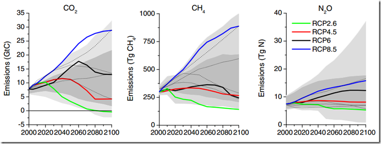
GHGEmissions

Figure 6, van Vuuren et al., 2011

The statement is repeated in a bullet point below E.1, along with the reference to where we can find more information in the heart of the report:

Relative to the average from year 1850 to 1900, global surface temperature change by the
end of the 21st century is projected to likely exceed 1.5°C for RCP4.5, RCP6.0 and RCP8.5
(high confidence). Warming is likely to exceed 2°C for RCP6.0 and RCP8.5 (high confidence),
more likely than not to exceed 2°C for RCP4.5 (high confidence), but unlikely to exceed 2°C
for RCP2.6 (medium confidence). Warming is unlikely to exceed 4°C for RCP2.6, RCP4.5 and
RCP6.0 (high confidence) and is about as likely as not to exceed 4°C for RCP8.5 (medium
confidence). {12.4}

My Bold.  Based on my reading,  I think the current state of evidence makes it difficult to agree with the qualitative expressions of probability given for RCP4.5 ("more likely than not") and RCP6.0 ("likely") regarding the 2 degrees target, as well as the "high confidence" given, which I will explain in more depth below.

My interest in this was sparked recently when using a two-layer model with prescribed TCR and effective sensitivities to trace the warming up to the year 2100.  Somewhat surprisingly, I found that for many realistic TCR scenarios, the simulated earth warmed less than 2°C  by the end of the century.  I began to do a scan of the recently released AR5 to find the justification for the scenarios mentioned above.

2. Probabilistic Statements and Confidence

First, let’s discuss what the SPM means by "more likely than not to exceed 2°C for RCP4.5 (high confidence)".  Based on my reading of the Uncertainty Guidance, I believe this should mean there is more than a 50% chance of reaching 2°C by the end of the century ("more likely than not"), and that there is plenty of evidence that is in widespread agreement ("high confidence") about this probability.  Regarding the statement about RCP6.0, "Warming is likely to exceed 2°C for RCP6.0 and RCP8.5 (high confidence)", the "likely" refers to a greater than 66% probability.

Anyhow, since SPM points us to Chapter 12 (and section 12.4 in particular) that’s where I’ll start.  From section 12.4.1.1:

The percentage calculations for the long-term projections in Table 12.3 are based solely on the CMIP5 ensemble, using one ensemble member for each model. For these long-term projections, the 5–95% ranges of the CMIP5 model ensemble are considered the likely range, an assessment based on the fact that the 5–95% range of CMIP5 models’ TCR coincides with the assessed likely range of the TCR (see Section 12.4.1.2 below and Box 12.2). Based on this assessment, global mean temperatures averaged in the period 2081–2100 are projected to likely exceed 1.5°C above preindustrial for RCP4.5, RCP6.0 and RCP8.5 (high confidence). They are also likely to exceed 2°C above preindustrial for RCP6.0 and RCP8.5 (high confidence).

This seems to suggest that for the long-term projections (that is, the warming expected by the end of the century), this is based solely on the CMIP5 model runs.  The observational assessments of TCR (transient climate response) only come into play in so much as that “likely” range approximately matches the 5%-95% range of CMIP5 models.  Notice that the statement of greater than 2°C being “more likely than not” for RCP4.5 is absent right here, despite being present in the relevant portion of the SPM.  So how does that statement find justification in the SPM, and how does it have "high confidence"?

3. On the “More Likely Than Not / High Confidence” RCP4.5 Statement

My impression is that this statement arises based on table 12.3, where 79% of the models produce a warming of more than 2°C under the RCP4.5 scenario.  The high confidence presumably comes from the agreement between the assessed likely  range of TCR estimates and the 5-95% range of TCR in models, but the problem with this becomes obvious when looking at box 12.2, figure 2:

Box12.2_Figure2

Box 12.2, Figure 2

Note that while the assessed grey ranges roughly match, the actual distributions are largely different.  The CMIP5 models have a mode for TCR > 2 (with a mean of 1.8, per chapter 9), while most of the AR5 estimates show a mode to the left of it.  In other words, just because there is "high confidence" in the 5% and 95% boundaries for CMIP5 projections, this does NOT give a legitimate basis for translating it into confidence about more specific aspects of the CMIP5 projected temperature rise distributions, particularly the "most likely" values (implied by the "more likely than not" statement).  Moreover, our best current evidence suggests the average of CMIP5 models is running too hot (as seen below), so one must be especially careful about making such specific statements based AOGCM results.

In section 12.4.1.2, the report alludes to the higher CMIP5 transient response issue:

A few recent studies indicate that some of the models with the strongest transient climate response might overestimate the near term warming (Otto et al., 2013; Stott et al., 2013) (see Sections 10.8.1, 11.3.2.1.1), but there is little evidence of whether and how much that affects the long term warming response.

This last statement is quite curious.  After all, the report claimed above that the rough matching of the range of TCR estimates with the 5-95% range of CMIP5 TCRs increased confidence in CMIP5 projections of long-term warming, but here the discrepancy in TCRs between estimates and models is dismissed due to lack of evidence of how it affects long-term warming? This seems hard to reconcile with Box 12.2, which notes:

For scenarios of increasing radiative forcing, TCR is a more informative indicator of future climate than ECS
(Frame et al., 2005; Held et al., 2010).

Indeed, this relative importance of TCR for end of century warming is one of the things I talked about in my last post Further investigation using that 2-layer model (script here) produces the following chart of TCR vs. 2081-2100 temperature above pre-industrial: 

RCP4.5

While the model is simplified and only uses one mean forcing series (from Forster et al., 2013), it indicates that a TCR less than 1.6 K likely indicates less than 2 degrees of warming by the end of the century for the RCP4.5 scenario.  Again, going back to table 12.3, we see that 79% of the models produce a warming of more than 2°C under the RCP4.5 scenario.  However, by my count, only 8 of the 31 models (26%) have a TCR of less than 1.6K, so this matches up decently with expectations based on TCR (although the picture isn’t quite that pretty, as 2 have TCRs of 1.6K).  Nonetheless, I would suggest that if the true TCR is less than 1.6K, the RCP4.5 scenario is unlikely to produce a warming of more than 2°C by the end of this century (relative to pre-industrial). 

Thus, our question comes down to this – given the best possible evidence, what is the probability that TCR is < 1.6K?  I would suggest it is "more likely than not".  First of all, it appears that the bulk of the AR5 estimates that include a pdf show a most likely value <= 1.6K.  This is despite the fact that (I believe) only Otto et al. include the lesser impact of aerosols assessed in AR5 in their estimate, which would further reduce the estimated likely values for TCR.  Second, it is generally accepted now that the multi-model mean, with its 1.8K TCR, is running on the warm side.  Either way, given the discrepancy between most-likely values in the various estimates, I would downgrade the confidence.

My rewrite of the SPM for this part: "Relative to the average from year 1850 to 1900, global surface temperature change by the end of the 21st century will more likely than not stay below 2°C for RCP4.5 (medium confidence)."    

4. On the “Likely” / “High Confidence” RCP6.0 Statement

Things start out a bit confusing for the "likely"  greater than  2°C statement for RCP6.0, per the following comment under the chapter 12 executive summary notes:

Under the assumptions of the concentration-driven RCPs, global-mean surface  temperatures for 2081–2100, relative to 1986–2005 will likely
be in the 5–95% range of the CMIP5 models

(My italics)  I say that this is somewhat confusing because a 5%-95% range – according to the chapter  – is associated with "very likely", and not simply "likely".  However, we must distinguish between the range of model outcomes and that of real world possibilities, which the authors appear to do as well.  Given that the assessed "likely" range of TCR is approximately as wide as the 5%-95% TCR range of the CMIP5 models, it is clear that some sort of probabilistic downgrade is required (that is, using only 1 standard deviation of CMIP5 model TCR does not properly capture the whole "likely "range of real-world TCRs).  So the authors assess that the "very likely" range of CMIP5 models is only expected to capture the "likely" range of real-world possibilities (Sect 12.4.1.2 again):

The likely ranges for 2046–2065 do not take into account the possible influence of factors that lead to near-term (2016–2035) projections of GMST that are somewhat cooler than the 5–95% model ranges (see Section 11.3.6), because the influence of these factors on longer term projections cannot be quantified. A few recent studies indicate that some of the models with the strongest transient climate response might overestimate the near term warming (Otto et al., 2013; Stott et al., 2013) (see Sections 10.8.1, 11.3.2.1.1), but there is little evidence of whether and how much that affects the long term warming response. One perturbed physics ensemble 
combined with observations indicates warming that exceeds the AR4 at the top end but used a relatively short time period of warming (50 years) to constrain the models’ projections (Rowlands et al., 2012) (see Sections 11.3.2.1.1 and 11.3.6.3). Global-mean surface temperatures for 2081–2100 (relative to 1986–
2005) for the CO2 concentration driven RCPs is therefore assessed to likely fall in the range 0.3°C–1.7°C (RCP2.6), 1.1°C–2.6°C (RCP4.5), 1.4°C–3.1°C (RCP6.0), and 2.6°C–4.8°C (RCP8.5) estimated from CMIP5
.

My bold.   (Note that the chapter indicates 0.6°C as the difference between pre-industrial and 1986-2005, so the RCP6.0 range is 2.0°C–3.7°C above pre-industrial, as confirmed in table 12.3). 
 
So, what are the problems here?

First, this seems awfully casual about the divergence between model projections and observed temperatures.  I understand that it may be unclear about how this relates to long-term projections (although several recent observational studies find a lower ECS than most model CMIP5 ECS’s as well), but this should not then translate into "high confidence" in the CMIP5 projections, particularly the lower end of that range.

Second, the assessed "likely" TCR range includes TCR values that would probably keep the RCP6.0 scenario below 2.0°C by the end of the century.  Note that the floor of the RCP6.0 range for CMIP5 is exactly 2.0°C above pre-industrial, which is presumably why the executive summary was able to say warming will "likely" be above 2.0°C for that scenario, but just barely.  Again, the confidence is "based on the fact that the 5–95%  range of CMIP5 models’ TCR coincides with the assessed likely range of the TCR".  But the ranges don’t match exactly, per Box 12.2 again:     

This assessment concludes with high confidence that the transient climate response (TCR) is likely in the range 1°C–2.5°C, close to the estimated 5–95% range of CMIP5 (1.2°C–2.4°C, see Table 9.5).

So the lower end of the "likely" range of TCR is 1.0°C (all evidence) rather than 1.2°C (CMIP5 only).  This would be a rather trivial difference, except that the lower floor for projected "likely" range using CMIP5 for RCP6.0 is exactly 2.0°C, so that lowering this 5% range to reflect all evidence – even if only from 1.2°C to 1.0°C – means probably lowering that projected warming above pre-industrial floor to around 1.7°C (1.0/1.2 * 2.0).  In other words, the "likely" range actually includes values below 2.0°C, and it would be difficult to say that that rise for RCP6.0 is "likely" to be above 2.0°C.***

Moreover, as you can see from my simple two-layer model tests below, a TCR <= 1.4K would mean we would probably see less than 2.0°C in this scenario:
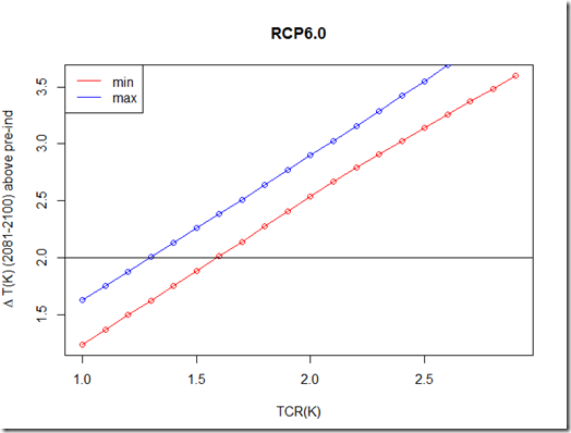
RCP6

Obviously, there is not much to suggest that the possibility of a TCR <= 1.4K is "unlikely", particularly when examining Box 12.2, Figure 2.  What’s more, the Otto et al. estimates, which are (I think) the only ones listed to use the AR5 aerosol estimates, indicate the "most likely" value is in this range!  So we are left in the rather awkward position that one of the more high-profile studies, using the most up-to-date data, suggests a "most likely" value for TCR that implies less than 2.0°C warming by the end of the century for RCP6.0, but the executive summary says that there is "high confidence" that greater than 2.0°C warming is "likely".

Third and finally, note that the "likely" ECS range in AR5 includes 1.5 K (Box 12.2, fig 1).  Now consider that the "effective forcing" for the RCP6.0 scenario above pre-industrial is 4.8 W/m^2.  This means, that at an ECS of 1.5K, you would only have 1.9°C of warming (4.8/3.7 * 1.5) at equilibrium (which can take several centuries to reach), regardless of the TCR.  Given the time delay to reach that equilibrium, it is probable that any ECS below 2K is unlikely to produce more than 2°C of warming by the end of the century in the RCP6.0 scenario.  Thus, the "likely" statement for more than 2°C in RCP6.0 is again questionable, even if based solely on the AR5 likely range of ECS estimates.

One more thing I want to address is the fact that in table 12.3, 100% of the RCP6.0 model runs produce a temperature rise greater than 2°C, despite 5 of the CMIP5 models having a TCR <= 1.4K.  From what I can tell, FGOALS-g2 (1.4K TCR) and INM-CM4 (1.3K TCR) didn’t participate in the RCP6.0 runs.  For the other three models (GFDL-ESM2G, GFDL-ESM2M, and NormESM1-M), I would have expected (based on their TCRs alone) to see less than 2°C of warming, and can only offer a few possible explanations: a) The ECS values of 2.4, 2.4, and 2.8 for these models are high relative to what one might expect for their low TCR values (failing to touch the lower end of the assessed "likely" range for ECS), and despite the greater importance of TCR, the higher ECS in this case might have pushed them just over the 2C mark, and/or b) these models may have produced an "effective forcing" for the RCP6.0 scenario greater than the 4.8 W/m^2 from the model ensemble.       

My rewrite of the SPM for this part: "Relative to the average from year 1850 to 1900, global surface temperature change by the end of the 21st century are as likely as not to exceed 2°C for RCP6.0 (low confidence)."    

***Note I say "difficult" rather than "impossible", because if the "likely" range include the middle 67% (approximately +/- 1 standard deviation), then excluding a low value from this likely range actually suggests about an 84% probability of it being greater than this value, not simply the 67% required to get to "likely".  However, more discussion / justification would certainly be required about performing a one-tailed test to deem a value "unlikely". 

5. Discussion

While I disagree with these particular statements in the SPM regarding the current best evidence, I find it hard to fault the authors, as I think much of the problem results from the IPCC process.  Essentially, with the projections based almost entirely on the CMIP5 models, and the IPCC unable to present any “novel” science that doesn’t appear published elsewhere (and hence produce new projections), it is hard to incorporate various other estimates of TCR and ECS into these projections.  Moreover, one is forced to consider most (or all) studies regardless of quality and even if using outdated data.  In fact, I think the authors made a wise decision to avoid using the 5%-95% range from CMIP5 as “very likely”, instead downgrading it as “likely” to reflect the spread of estimated TCRs and ECSs.  Unfortunately, this still has implications on the edges (as with the RCP 6.0 lower boundary of 2°C instead of 1.7°C) and center (trying to figure out a “most likely” value for RCP4.5).  Moreover, we have a rather awkward situations where “likely” values of TCR and ECS imply less than 2°C warming for RCP6.0, but we the SPM says that there is “high confidence” in a “likely” diagnosis for more than 2°C warming under RCP6.0.

Overall, I do not envy the job of the IPCC authors, and tend to agree that producing these massive reports for free is probably not the best use of anyone’s time.  It might be better to just create a “living” document such as a wiki, as others have suggested, although I can only imagine the struggles one would come up with in determining the rules for that.

6. Summary

In my opinion, the IPCC summary for policymaker’s overstates both the probability and the confidence in hitting the 2°C target by the end of the century for the RCP4.5 and RCP6.0 scenarios.  This is because:

  • The statements about the probability were based primarily upon CMIP5 projections
  • Confidence in these long-term projections was primarily justified by the 5%-95% range of CMIP5 transient climate responses (TCRs) matching up with the assessed likely range of TCRs from a variety of other sources, yet
  • Where the real-world transient responses began to diverge from models, this was not determined to decrease confidence in the long-term range of projections, and
  • Confidence in the 5%-95% range of CMIP5 TCRs was deemed to imply confidence in the “most likely” (50%) CMIP5 projections for RCP4.5, despite the AR5 “all-evidence” assessed TCR having a largely different distribution than that of the CMIP5 TCRs.
  • Despite the fact that several assessed “likely” values for TCR imply less than 2°C warming for RCP6.0, it was still determined that there was “high confidence” that greater than 2°C warming was “likely” for RCP6.0
  • Despite the fact that several assessed “likely” values for equilibrium sensitivity (ECS) imply less than 2°C warming for RCP6.0, it was still determined that there was “high confidence” that greater than 2°C warming was “likely” for RCP6.0
Older Posts »

Create a free website or blog at WordPress.com.