CMIP5 Effective Sensitivity vs. Radiative Response in Last 40 Years

This post forms part 2 of the series I started in the last post, which focused on using the energy balance over the period of 0-2000m OHC data to estimate sensitivity.  As you recall, I noted that using the radiative response over this shorter period actually overestimated temperature sensitivity in the GISS-ER and GFDL CM2.1 model runs, so I wanted to test how the radiative response over this shorter period compares to the “effective sensitivity” in all the CMIP5 runs. 

1. Effective Sensitivity in CMIP5 Runs

Note that I am using “effective sensitivity” here in the sense of Soden and Held (2006)…the net radiative response to an increase in surface temperature over a long term scenario (units W/m^2/K).  In my specific case, I am using the RCP4.5 scenario runs from the CMIP5 models, which hold fixed a 4.5 W/m^2 anthropogenic forcing change in 2100.  In addition to the forcing difference, I use the difference in net radiative imbalance and temperature between the two periods 1860-1880 and 2080-2100. 

The data I grabbed from Climate Explorer using a script (you’ll need to register and insert your own e-mail address), which I developed with some help from this Climate Audit post that cut down the learning curve.  This is not a complete set of all CMIP5 models available at Climate Explorer at the time, as some seemed to be missing radiation fields and others caused my script to choke, but it is *almost* all of them.  Anyhow, here are the diagnosed “effective sensitivities” in the individual model runs (note again that if you were assuming a constant radiative response, you could determine the equilibrium climate sensitivity based on 3.7/effective_sensitivity):

I have not compared these results to Andrews et al. (2012), but if anybody has a copy of this paper I would love to do so.  Anyhow, as you can see, each of the model runs are pretty tightly clustered with other runs within the model, which is to be expected.  One exception was CESM1-CAM5, but after looking at several of the runs it was clear that they had an offset in the splicing of the beginning of the RCP4.5 run onto the end of the historical run.  Looking at this chart again, I’m noticing something suspicious in one of those CCSM4 runs, with 5 runs very closely clustered and then 1 “rogue” one.  I will need to check if that is an offset error as well.  Anyhow, here is a look at the mean “effective sensitivities” and number of runs for each model:

 

2. Shorter-Term Radiative Response (from last 40 years) in CMIP5 Runs

In order to test the method I used in the last post, here we will determine the radiative response based on the difference (in TOA imbalance and surface temperature) between the the 2005-2011 period and the 1965-1974 period.  The latter period was determined by finding the best correlation between the resulting radiative response diagnosed for the models and the longer “effective sensitivity” for those same models. 

One huge difficultly with determining this radiative response for a model is that the TOA forcing data is simply not available (at least, in my experience).  It requires a special fixed SST run to do this calculation***, and I don’t believe this is included in the CMIP5 archive.  Thus, I have decided to simply use the GISS forcings for ALL the calculations, and this will cause some slight inaccuracy in the diagnosed radiative response for other models.  Nonetheless, here is the radiative response as diagnosed:

For reference, using the GISS estimate for the aerosol forcing (and not the IPCC one, which is of smaller magnitude), my test in the previous post resulted in a –2.4 +/- 0.8 W/m^2/K response over this same period, which is a good deal stronger than most model runs.  

***The Forster and Taylor (2006) method uses the inverse of the long-term radiative response to estimate forcing, but we can’t do that here because we are testing the relationship between the shorter-term and long-term response, and the assumption that these would be the same would be begging the question. 

3. Relationship between 40 year Radiative Response and Effective Sensitivity

The plot below shows the relationship between the 40-year response and the effective sensitivity.  The r^2 value is 0.36, which is pretty strong despite the fact that I have essentially ignored the difference in aerosol forcing between the models. 

So, what can this knowledge, combined with the previous test, tell us about effective sensitivity of the real world system?  The chart below includes red lines showing the least/likely/most radiative response from observations over that same period (–2.4 +/- 0.8 W/m^2/K, again assuming GISS forcings rather than the IPCC): 

If we were confident in that regression, our “likely” estimate for “effective sensitivity” would be right around –2.0 W/m^2/K, which would correspond to an ECS of ~ 1.85 K if we assumed a negligible difference between the “effective sensitivity” radiation response and that response over the full time it takes to equilibrate.   However, I don’t think much stock can be placed in that regression, given that we have not used particularly accurate forcing data for the individual model aerosols, and the radiative response is well outside the main cluster of models.  I think this latter fact is the more interesting qualitatively – there IS a fairly strong underlying relationship between this 40 year radiative response and the longer term “effective sensitivity”, and only 3 model runs of all the model runs looked at here have this radiative response fall within the 2.5%-97.5% uncertainty range as diagnosed from OHC in my last post.  Of those, 1 of those “compatible” runs is a rogue CCSM4 run that is almost certainly affected by an offset issue.  I am curious about the other 2 models/runs that diverged from the pack as well, but these don’t seem likely to be “rogue” runs because their corresponding effective sensitivities (which would also be affected by an offset issue) are normal.  Regardless, given that the modeled aerosol forcings tend to be larger in magnitude than in satellite estimates, this line of evidence would suggest it is even more likely that the effective temperature sensitivity of almost all CMIP5 models is too high.

This presents an additional test to just comparing temperature trends to models, because temperature and radiative imbalance will be negatively correlated if all else is kept equal.  So in the event that you get a lower temperature trend in the real world than models due to La Nina conditions towards the end of the period, you should see an increase in TOA imbalance relative to models as a consequence of this unforced cooling, assuming the radiative response between the real world and models are about the same.  However, as both the temperature trend AND TOA imbalance trend are smaller than almost all CMIP5 models over this period, La Nina would not serve to explain the situation.  This leaves some combination of the following possibilities that I can see: 1) incorrect diagnosis of TOA imbalance from 0-2000m OHC, 2) aerosol forcing greatly exceeds that of GISS (which itself greatly exceeds the IPCC best estimate), 3) some other unknown forcing, 4) too high of effective temperature sensitivity in the CMIP5 models.    

Data and Code

The following script, ProcessCMIP5Data.R, accesses the CMIP5 data in my public folder and creates the figures for the above post.  HOWEVER, it is quite a few files, and processing will be slow if you run the above turnkey script.  Instead, I recommend you download the data to your local machine first, unzip it, and then change “baseURL” in the above script to point to your specific folder you unzipped it into.

Estimating Sensitivity from 0-2000m OHC and Surface Temperatures

1. Introduction

This post should be the first in a series covering how we might derive an "empirical" estimate for climate sensitivity from ocean heat content (OHC) and surface temperature changes.  I’ve touched on this topic a few times in previous posts, but my goal for this one is to have it be a more thorough examination. 

The basic equation I want to use here is one we’ve seen quite a few times before:

ΔN = ΔF + λ*ΔT

Here, N is the TOA radiative flux, F is the forcing, T is the surface temperature, and λ is the radiative response term, also referred to as "effective sensitivity" in Soden and Held (2006) and "climate feedback parameter" in Forster and Gregory (2006), both of which can be confusing as they mean slightly different things than "sensitivity" and "feedback" in current climate lexicon.  For more information you can see my page here,  although I think parts of that may out-of-date enough to not totally reflect my evolving views.  For instance, I see more and more evidence that this radiative response to inter-annual fluctuations is a poor predictor of the radiative response on the climate scale.  This is why I hope to use differences in longer periods — e.g. 30 years — to determine a more relevant value for λ.  Of course, we don’t have a single satellite that runs that long to compare TOA imbalance, but we can estimate it…from the OHC data. 

One other thing worth mentioning here is that while theoretically it should be possible to determine the equilibrium climate sensitivity (temperature change with a doubling of CO2) by simply dividing the forcing (~3.7 W/m^2) by the radiative response, this assumes that λ is a constant for different timescales and forcing magnitudes, which is far from true in some models (whether this departs significantly from constant in the "real world" system is debatable).  Winton et al. (2010) refer to this in terms of "Ocean Heat Uptake Efficacy", and Isaac Held has a discussion of it on his blog. .  Paul_K also discussed this at The Blackboard.  This is why the dividing the CO2 forcing by "effective sensitivity" in Soden and Held (2006) calculated from 100 years of the A1B scenario does not directly match the equilibrated temperature change from the idealized CO2x2 scenario.  While the latter may be near impossible to accurately determine without thousands of years of well-constrained observations, the former is arguably much more useful anyhow, so I’ll set my sights on that.

2. Forcing Uncertainty

The start of the NOAA OHC data is 1955, so estimating the TOA imbalance from this data means we’re limited to 1955 and on (actually a bit later, but we’ll discuss that in the next section).  So, what kind of forcing uncertainty are we looking at over this period?  For this, we can first take a look at the GISS forcings, derived in the method described from Hansen et al. (2005), which are also very similar to the AR4 time evolution of forcings modeled using MIROC+SPRINTARS.  Similarly, I digitized the GFDL CM2.1 forcing evolution from Held et al. (2010), and we get something similar.  Moreover, since the emissions histories are all very similar, it seems the differences in these forcing histories can largely be determined based simply on an "aerosol efficacy factor" for anthropogenic aerosols.  Here is a reconstruction of the GFDL CM2.1 forcing history from the GISS forcings, but using an "efficacy" of 0.75 for anthropegic aerosols:

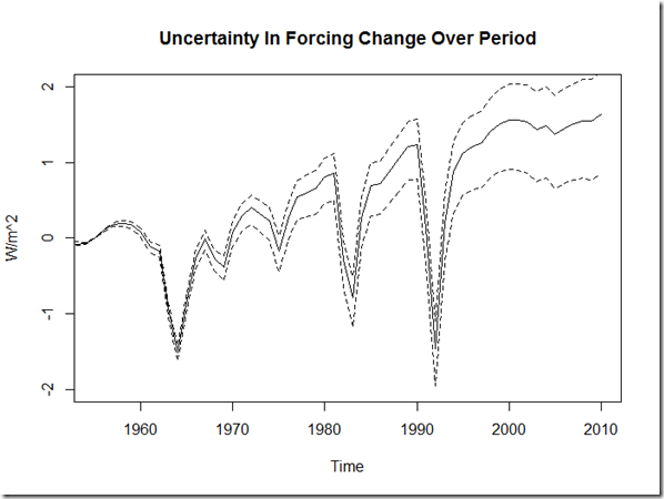
As you can see, it is a pretty solid match.  Thus, in order to determine the potential forcing histories used for “observations” in this experiment, I take the bounds for present-day aerosol estimates and compare that to the GISS forcing, and then use this factor for efficacy.  The AR4 estimate for direct aerosol forcing is -0.5 +/- 0.4 W/m^2, and for indirect it is a most likely value of -0.7 W/m^2, with 5% to 95% range of -0.3 to -1.8 W/m^2. .  From 1955, this produces the following uncertainty bounds for forcings if we use an aerosol forcing from -0.4 to -2.3 W/m^2:

With Monte Carlo, we can use a Gaussian distribution for the direct aerosol forcing and a triangle distribution for the indirect effect to get the following distribution for combined aerosol forcing difference (1955 – present day):

 

3. Inferred TOA Imbalance

As the measurements are very sparse down to 2000m prior to 2005, Levitus et al. (2012) provides only pentadal averages for OHC in the 0-2000m depths over that time period.  We can calculate the approximate 5 year average TOA imbalance using the difference in 5 year OHC averages.  For example, we estimate the 1957.5-1962.5 average TOA imbalance by subtracting the 1955-1959 average from the 1960-1964 average (the conversion from differenced Joules of 5 year averages to global average flux is ~0.124).  However, we also need to note that not all of the extra energy is stored in the 0-2000m of the ocean…some goes into the atmosphere, into the cryosphere, or into the deeper ocean, so we’ll need to multiply this by some factor.  We can use output from GCMs to estimate how well this method works:

First, for GISS-E2-R, a regression suggests only about 70% of the heat goes into this 0-2000m layer, but the reconstruction is quite good:

For GFDL CM2.1, the amount of heat is stored in 0-2000m ocean is about 85% of the imbalance, which seems more realistic.  Levitus et al. (2012) estimates that 90% of the heat has gone into the ocean.

For a comparison of the 5 year running averages of OHC 0-2000m between the CMIP5 GFDL CM2.1 runs and the GISS-E2-R runs and the NOAA observations, I downloaded a bunch of ocean temperature data by layer from two different Earth System Grid Federation nodes: here and here.  PLEASE NOTE: that this is NOT raw output data from the models, and it took a good amount of time on my part to download and process the data from the freely available kernel ocean temperatures into global heat content, so if you are using the data in the form I make available here (you can see the links in the scripts) I would request you acknowledge here as the source. 

Additionally, NOAA provides 1 year averages for OHC 0-2000m from 2005.5-2011.5.  By calculating the current imbalance using annual differences based on a regression dOHC/dT, we can estimate our imbalance up to the most recent full year.

4. Estimating Radiative Response Term using Monte Carlo

There are a number of uncertainties present, and to see their net effect I use Monte Carlo with 1000 iterations for each start year, from 1957 to 1985.  The prior distribution for the forcing change was described in section 3.  For estimating the heat going into the 0-2000m layer, I use a Gaussian distribution with standard deviation equal to the published standard error (from Levitus et al. 2012) for each year, with the OHC value for that year obviously centered on the most likely value presented in that data.  This is then diff’d to determine the change in OHC, and converted into TOA imbalance by sampling from a uniform distribution that assumes 75%-85% of any heat imbalance is stored in that 0-2000m layer.  Except for the “current” imbalance from 2005-2011, where the values are better constrained, I use 10-year averages (rather than 5) to limit the uncertainty for each start year.

Ultimately, the “radiative response” is determined from ((N2-N1)-(F2-F1))/(T2-T1), where N2 is the 2005-2011 Imbalance, N1 is the ten year average imbalance from an earlier start year period (starting at the StartYear), F2-F1 is the difference in forcing between the most recent 8 years and the average forcing over the earlier 10 year period, and T2-T1 is the difference in surface temperature between the most recent 8 years and the average surface temperature over the earlier 10 year period (the temperature used here is an average between the GISTemp and NCDC temperature datasets).      

For those curious, the mean value I get for the TOA imbalance from 2005.5-2011.5 is ~0.57 W/m^2, which is pretty consistent with other estimates.
 

5. Results

The figure above shows the 2.5%-97.5% uncertainty (and median) for the observations, versus the span of 5 runs (and their median) for GISS E2-R and GFDL CM2.1.  A few things jump out: first, the uncertainty for GISS E2-R is extremely small even compared to GFDL CM2.1, which we could probably attribute to an underestimate of internal variability.  Second, that even though the error bars overlap for a number of periods, it would appear that these models underestimate the radiative response, suggesting that they likely overestimate climate sensitivity. 

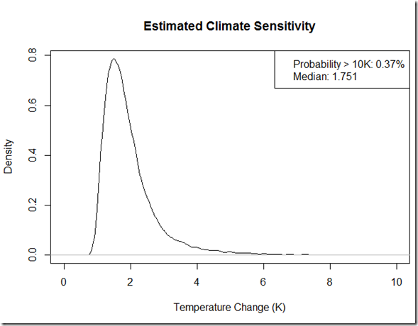
Now, for kicks, if I were to ignore the issue of λ not being a constant (and assuming it was the same for all forcings), I could flip this and get the following pdf for climate sensitivity. 

 

As you can see, such an approach yields “most likely” estimate of around 1.8 K that is outside of IPCC likely range.  However, this method in itself fails to constrain the extremely high sensitivities due to the scenarios where negative aerosols have almost completely offset GHG warming, leaving a potential of > 10 K at around 1 in 200.

Furthermore, the observant reader may have noticed that in the graphs of the two GCMs above, this method has actually overestimated the sensitivity.  The GISS ER CO2 doubling forcing is 4.06 W/m^2, but the median radiative response is only -1.11 W/m^2/K, yielding a sensitivity of 3.6 K that is greater than it’s known sensitivity of 2.7 K.  The median radiative response for GFDL CM2.1 using this method is merely –1.02 W/m^2/K, and with its 3.5 W/m^2 forcing this yields a sensitivity of 3.4 K that is almost its actual equilibrium sensitivity.  However, the latter is likely just luck, because the GFDL CM2.1 has an extremely high uptake efficiency factor that should cause an underestimate of the sensitivity in any short-term estimate like this.  One need only compare to the “effective sensitivities” in Soden and Held (2006) to see that this method underestimates the radiative response (-1.64 W/m^2/K and –1.37 W/m^2/K for GISS and GFDL respectively), and I’m not sure why exactly; my best guess at this point would have to do with the response to the high volcanic activity during this time period. 

I will compare the results we get here to those of other CMIP5 models in (hopefully) my next post in order to see how effective this method might be for determining century scale sensitivity.

UPDATE (10/27):

When running my script again for the most recent post, I noticed I had used the mean of the 2004-2008 forcings rather than 2005-2011 forcings for the recent period.  The change skews the PDF slightly to the left, but otherwise does not result in a huge change.  The script has been updated in the link below.  Here is the updated look:

Code

Please acknowledge any code or data used from this post.  Thanks!

Introductory Charts.

Monte Carlo Estimates.

References

Forster and Gregory (2006): http://journals.ametsoc.org/doi/pdf/10.1175/jcli3611.1

Soden and Held (2006): http://www.gfdl.noaa.gov/bibliography/related_files/bjs0601.pdf

Winton et al. (2010): http://www.met.igp.gob.pe/publicaciones/2010/efficacy[1].pdf

Hansen et al. (2005): http://pubs.giss.nasa.gov/docs/2005/2005_Hansen_etal_2.pdf

Held et al. (2010): http://journals.ametsoc.org/doi/abs/10.1175/2009JCLI3466.1

Levitus et al. (2012): http://www.agu.org/pubs/crossref/pip/2012GL051106.shtml

Hansen et al. (2011) http://www.columbia.edu/~jeh1/mailings/2011/20110415_EnergyImbalancePaper.pdf

Water Vapor and Temperature Feedbacks from recent warming patterns

I suppose this would be the third part in my series, as I would like to revisit my post from a month and a half ago, "Sensitivity of the water vapor feedback to locations of SST trends".   In that post I used the GFDL HiRAM180 AMIP runs to show that the effective water vapor feedback has likely been substantially less in the AMIP warming period (1981 – 2008) due to the bulk of the SST increase coming at higher latitudes rather than in the tropics.  Amid the caveats, I noted that "it is quite possible that some of the lessening of the positive water vapor feedback may be counteracted by a decrease in the strength of the negative lapse rate feedback which could mitigate the effect on overall sensitivity." 

As you can see from a figure like the one above from Soden et al. (2008, Journal of Climate), warming at higher latitudes will decrease the water vapor feedback, but so too will it decrease the outgoing OLR from the temperature response.  Thus, I wanted to see what degree the lesser water vapor feedback would be offset by this effect, and thus processed the atmospheric and surface temperature values from GFDL CM 2.1 and HiRAM 180 in the same way I’d done for water vapor.  Code and intermediate data available here.

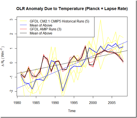
First, here is the OLR anomaly due to temperature changes:

As you can see, the increase in OLR is not nearly as high in the AMIP runs bounded by SST observations as it is in the fully coupled, CM 2.1 runs.   And when we combine the OLR anomalies from water vapor and temperature, we again see a lesser increase in the OLR anomaly (note that the y-axis units are smaller in this case than in the above chart):

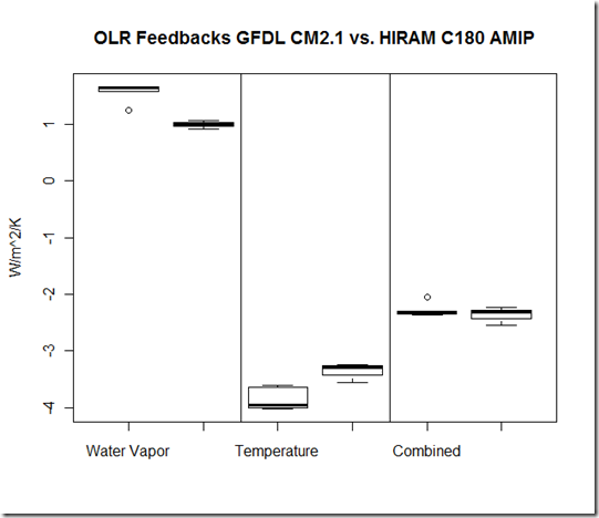
However, again keep in mind that we haven’t seen as much warming over this period as is present in the CM2.1 runs, and the effective feedback is going to have that temperature increase as the denominator.  So, here are the effective feedbacks for Water Vapor, Temperature, and then these two combined (CM2.1 comes first in each category):

Pretty interesting, at least to me.  The decrease in the negative temperature feedback for our actual warming pattern seems to totally offset the decrease in the positive water vapor feedback from that same pattern, such that the combined feedback are extremely close between the CM2.1 and HiRAM AMIP runs.