CERES and ERA-Interim fluxes in Dessler 2010

As I noted in a previous blog post, and as mentioned at Climate Audit, the positive cloud feedback results (and excluding large negative feedbacks) of Dessler 2010 (not to be confused with Dessler 2011, which was the topic of my latest post) largely depend on using ECMWF ERA-Interim reanalysis for the clear-sky fluxes rather than CERES.  The Cloud Radiative Forcing is determined by the difference between all-sky and clear-sky fluxes, and rather than using the CERES data for both clear-sky and all-sky, Dessler10 combines CERES all-sky with  ERA clear-sky.  The reason given for doing this is a suggested bias in the CERES clear-sky, with a reference to the Sohn And Bennartz 2008 paper.

In that first post, and in my guest post at Lucia’s, I pointed out two things:

1) The largest amount of this difference seems to come from the shortwave fluxes, which are unaffected by this longwave water vapor bias, and

2) Even if the OLR dry-sky bias was present, it would not account for the differences we see here:

But I’m doubtful that the LW result should be discounted based on measurement bias anyhow. For one, the SB08 paper refers to bias in the absolute calculation of CRF, not necessarily to the change in CRF, and the effect is minimal there (around 10% of only the OLR). Second, the bias should affect it in the opposite direction – it would make the cloud feedback appear more positive, not negative. From the SB08 paper, they mention: “As expected, OLR fluxes determined from clear-sky WVP are always higher than those from the OLR with all-sky OLR (except for the cold oceanic regions) because of drier conditions over most of the analysis domain.” Obviously, clear-sky days don’t prevent as much OLR from leaving the planet as cloudy days, and SB08 estimates that about 10% of this effect is from water vapor instead of all of it being from clouds. So, warmer temperatures should increase water vapor, which will be more prevalent on the cloudy days vs. the clear sky days, which in turn will make it appear that clouds are responsible for trapping more OLR than they actually do. In other words, the bias includes some of the positive feedback due to water vapor – which is already counted elsewhere – in the estimation of cloud feedback.

Now, Nick raised a point over at CA, that perhaps all we’re getting with ERA-Interim clear-sky fluxes is the CERES fluxes, but with this dry-sky bias removed:

What the reanalysis can then do is make the moisture correction so the humidity is representative of the whole atmosphere, not just the clear bits. I don’t know for sure that they do this, but I would expect so, since Dessler says that are using water vapor distributions. Then the reanalysis has a great advantage.

While I don’t believe this could be reconciled with either of the two points above (there is no dry-sky bias to "correct" in the shortwave fluxes, and the correction should be in the opposite direction), I want to give this a fuller treatment that should prove that the positive cloud-feedback result in Dessler10 is largely an artifact of combining the two different datasets.

If our hypothesis is that ERA_CRF is simply CERES_CRF corrected for dry-sky bias, we would be able to detect it rather easily be checking the relationship between the measured water vapor (total precipitable water from CERES) and the CERES_CRF-ERA_CRF differences.  The following scatter plot shows that relationship:

As you can see, the "dry-sky bias correction", if it exists in ERA, accounts for very little of the difference we see between ERA_CRF and CERES_CRF.  Please note the following point I made on that CA thread: 

Since we’re calculating CRF as the difference between clear-sky and all-sky fluxes, ANY difference in those two datasets is going to show up in the estimated cloud forcing, including their different estimates of solar insolation (which has nothing to do with clouds).  The magnitude of the changes in flux is far smaller that the magnitude of the total flux, so you would expect using two different datasets to have a lot more noise unrelated to the CRF. Note that if there is ANY flux calculation bias in either of the two datasets unrelated to clear-sky vs. all-sky, it WILL show up in the CRF, whereas if you use the same dataset, even if a flux calculation bias is present, it will NOT show up in CRF unless it is related to clear-sky vs. all-sky.

I’d like to pause a moment and note that the Dessler10 references to the ability of models to calculate clear-sky flux only refer to that of longwave flux.  This is because the shortwave flux is rather trivial, assuming you know the incident solar radiation and albedo:

outgoing_sw_clr = incoming_sw * albedo_clr

Of course, there is no definitive monthly value for albedo and incoming solar radiation, as evidenced by the fact that CERES and ERA have different values for these.  Albedo_clr is primarily just surface_albedo, although there is perhaps some aerosol mixed in.  This next chart shows the effective clear-sky albedo, which can be calculated from outgoing_sw_clr/incoming_sw, but it could just as easily be put in terms of the differences in clear-sky short-wave fluxes:

Well, there you have it.  The bulk of these CERES_CRF vs. ERA_CRF differences come from this different value for the effective surface albedo.  Note that this has nothing to do with a "dry-sky" longwave water vapor bias.  The value of 275?  That is approximately incoming_sw * (1 – cloud_albedo), as we’d expect when calculating the flux difference between net and clear-sky with no cloud albedo change.  I repeat, when combing the CERES all-sky flux with the ERA clear-sky flux, your “CRF” change will about equal to 275 * (CERES_surface_albedo-ERA_surface_albedo), even when no cloud properties have changed.  This is what I mean by slight differences from either set showing up as a bias in the CRF estimate when you combine them. 

Does it matter whether CERES surface albedo or ERA surface albedo is more correct?  Not at all, as long as they’re consistent.  You can make the corrections to the CERES short-wave all-sky flux to use the ERA surface albedo, or you can make the corrections to the ERA short-wave flux to use the CERES surface albedo, or you can just use CERES fluxes for both all-sky and clear-sky.  But the important thing to note here is that by combining the CERES all-sky with ERA clear-sky, you get a difference in what is effectively surface albedo bundled in with the CRF term, despite having nothing to do with clouds. 

Using HadCRUT with the CERES_CRF, I get a value of -0.50 W/m^2/K for the cloud feedback.  Using HadCRUT with the ERA_CRF included in Steve’s file from Dessler, I get a value of 0.26 W/m^2/K (This is slightly lower than the Dessler10 paper because additional adjustments are made to go from CRF to R_cloud from radiative kernels, which I’m not disputing here).  Correcting for the different effective surface albedos in the ERA_CRF, I once again get a negative value of -0.34 W/m^2/K.  None of them have much in the way of correlations.

I have previously suggested why we likely see lower correlations here, and how to correct it, and so I consider -0.34 W/m^2/K to be an underestimate of the short-term cloud feedback.  Nonetheless, to me there seems to be little ambiguity that the magnitude of the positive feedback in Dessler10 is more of an artifact of combining two flux calculations that aren’t on the same page, rather than some bias correction in ERA-interim.  I would welcome any comments to the contrary. 

The script I used for this post, along with some intermediate ERA data and the original CERES data, is available here.  To get the ERA-Interim raw data, you’ll need to use the synoptic means, grabbing the data at time steps of 12 hours, with times chosen of 0:00 and 12:00, for the months 2000 through 2010, and selected variables of at least incidental solar radiation and the top net solar radiation for clear-sky.

Thoughts on Dessler 2011

As I’ve already looked at SB11 in a previous post, now I’ll turn to Dessler 2011, also including the critique Dr. Spencer put up on his blog.  This post will just be dedicated to the “Energy Budget Calculation” section of D11, since there is plenty to go over there.  All data and code used in this post are available here.

First, I’ll include a couple representations of the same equation.  The first is from the Dessler’s video on his 2011 paper, and the second is from Spencer’s blog.

 

The unknown radiative forcing is represented by R in the Dessler equation, and N in Spencer’s.  S and F_ocean are also the same, and this term represents the unknown non-radiative forcing; that is, the flux coming in and out of the deeper ocean layers into the mixed layer (thereby “forcing” surface temperatures), or the flux coming in and out of the atmosphere (this is likely to be much smaller due to the lower heat capacity of the atmosphere).  The reason that Spencer has grouped the N – lambda*T terms together is because this represents the TOA flux, which is measured by CERES.

Criticism #1: The Mixed Layer Depth

Clearly, much depends on the value chosen for C, the heat capacity of the mixed layer.  This is proportional to the depth (since we’re adding more total mass the deeper we include), and so the depth chosen for the mixed layer is crucial.  Since we want to know to what degree surface temperatures are “forced” by energy fluxes from the deeper ocean layers, we need to know down to what depth the ocean temperatures are directly tied to the surface temperatures.  To determine this, I simply find the correlation between the sea surface temperature (Reynolds SST) and the ocean temperature at each depth (calculated in my last post).

Note that I’m using the CERES era here (2000-2010).  For our effective “global” mixed layer (hah!) , it appears to be somewhere between 50 and 75 meters.  I also want to pause and just note the curious spike at around 200 meters as well…I’m wondering if this has anything to do with the depth with which the energy from ENSO upwells, but that is for another time.  

Anyhow, Spencer uses 25m for this effective mixed layer, which looks to be too low.  Dessler says that he uses value of 168 W-month/m^2/K, which is the same as Lindzen and Choi 2011 and is a depth of 100 m, but as we’ll see later (and Spencer notes), it appears he is using an actual depth of 700m.  100 meters is likely on the high side, but 700 meters is way beyond what could be considered the mixed layer in this case.

Criticism #2: The Error Terms

In the equation above, we calculate S (or F_ocean) by subtracting the CERES-measured TOA flux anomaly from the difference in ocean heat content (down to the mixed layer depth, divided by the time step).  Each of these measurements (from CERES and Levitus) are bound to have some error, but the way we calculate S, all of this error is aliased into the non-radiatively forced term!  Since we’re comparing magnitudes by taking the standard deviations in S, there need not be a long-term bias in either measurements to cause a bias in S…I believe even random white noise will do it (I may give this a shot with some synthetic data). 

Running the Numbers

Now, in the Dessler paper, he mentions that he gets a standard deviation for F_ocean of 9 W/m^2 and 13 W/m^2 for monthly flux anomalies.  My first thought was that this appears to be quite a large number(~3 times what you get for a CO2 doubling), and that surely this would mean we’d see more than the ~ 0.1 K (standard deviation) surface temperature fluctuations over this time, even though the fluxes are short-term.   For my numbers, for 700m, I got about 5.14 W/m^2, which we could maybe reconcile by the fact that I only have 3-monthly anomalies available, and if Dessler didn’t remove the seasonal components over this CERES time period.  However, 700 meters CANNOT be used as the mixed layer depth.  As we can see above, or in my last post, the temperature down to 700 meters does not represent the surface temperatures (r^2 ~ 0.05), which we are using to diagnose the climate feedbacks.  This is why those flux anomalies don’t appear reasonable and do not show up in surface temperature fluctuations.  Using the incorrect 700m flux, I can get a ratio of about 10/1 for sd(S) / sd(N), which is on Dessler’s magnitude:

I’m presuming this is a simple mistake on Dessler’s part, using the 700 meter depth instead of 50 or 100 meter.  However, the following quote from Dessler 2011 gives me pause:

The formulation of Eq. 1 is potentially problematic because the climate system is defined to include the ocean, yet one of the heating terms is flow of energy to/from the ocean (F_ocean). This leads to the contradictory situation where heating of their climate system by the ocean (F_ocean > 0) causes an increase of energy in the ocean (C(dTs/dt) > 0), apparently violating energy conservation.

This appears to be a fundamental misunderstanding about the equation.  C(dTs/dt) represents the change in heat capacity of the mixed layer, while F_ocean represents the flux to/from layers below (deeper ocean) and above (the atmosphere).  There is no violation of energy conservation.  Furthermore, Dessler’s conflating the mixed layer ocean with the deeper layers of the ocean (considering both terms simply “ocean”), may have led to the mistake of including all 700 meters depth for the “mixed layer”.

To put it another way, we don’t care about the exchange of heat among ocean layers in this case UNLESS they are forcing surface temperature changes.  Since the depths below 100m are not tied to the surface temperature changes, the heat exchange from the (for example) 900 m and 700m level should NOT be included in the non-radiative flux term (S) unless it crosses that 100 m barrier, but Dessler’s formulation has included it (assuming he’s using 700m).  Furthermore, according to this formulation, ENSO would have no effect on surface temperatures if it caused warm water from the 200m to 700m layer to upwell into the surface layers, so the S term does not even seem to include the major effects of ENSO, which is the primary component of non-radiative forcings over this period!

Anyhow, for my three-month standard deviations in fluxes I get 1.85 W/m^2 for 100 meter depth, which is slightly less than the 2.30 W/m^2 that Spencer calculates.  This leads to ratios of between 3.2:1 and 3.8:1 for S/N, much less than Dessler’s number (20:1).  However, Spencer mentions on his blog that he gets a ratio of ~ 2:1 for the 100 meter depth, which I am unable to reproduce.

 

If we use the 50 meter depth, which is on the lower end for mixed layer depth choices, I get a flux standard deviation of about 1.08 W/m^2, and THEN I get a ratio of about 2:1:

This matches up with the Lindzen Choi 2011 paper, but is still a good deal larger than the SB11 estimate of 0.5:1.  As I mentioned above, the standard deviation of S might be inflated by errors in the CERES and/or Levitus data, but I doubt it is to that degree.  I’ll need to look into that later.

Anyhow, I went back to the Spencer-Braswell 2011 model and saw what effect it would have if we used the updated ratio calculations:

All of the lines, except the purple one, were generated using the ratios mentioned above for the 100 meter and 50 meter layer results.  In each case, the feedback is underestimated at zero lag.  However, note that none of ratios gives the lagged signature we see in the observations, except for the purple line, which requires that ratio of about 0.67:1 to get there.  From what I can tell, that would require a rather large combined error contribution from CERES + Levitus for that relationship to be true. 

So, in the interest of finding common ground between Dessler and Spencer, I would tentatively say the following (I reserve the right to change my mind if more information becomes available [i.e. I am shown to be wrong ]):

1. Part, but not most, of the surface temperature fluctuations in the last decade have come from unknown radiative forcings (25% – 40%).
2. This has led to underestimates of the overall climate feedback using CERES and surface temperatures, and has thus led to overestimates of climate sensitivity using this method.
3. The difference in the lagged signatures between the observations and GCMs are more likely the result of improperly modeled ENSO variations than they are the result of unknown radiative forcings.  (pending further review of the rest of Dessler 2011) . 

Update 9/19

For those of you questioning whether Dessler11 actually does incorrectly include all the way down to the 700 meter layer for his Argo data calculations, note the following from this paper:

This can be confirmed by looking at the Argo ocean heat concent data covering 2003-2008.  Using data reported in Douglass and Knox [2009], the month-to-month change in monthly interannual heat concent anomalies can be calculated (sd = 1.2 x 10^22 J/month).

The reference leads to this paper, which notes under section 3.1:

A new system was deployed in 2000 consisting in part of a broad-scale global array of temperature/salinity profiling floats, known as Argo [20]. Monthly values of Argo HO were determined from data to a depth of 750 m. Values from July 2003 to January 2008 are given by W08 and are listed in Table S-1.

Bold is mine.  If you have paywall access, you can simply download the supplementary data for table S-1, use the Argo columns, diff them (to get the change in OHC) and remove seasonal effects, and you’ll get the value of 1.2 for the standard deviation that Dessler gets above.  I would also note that it appears Dessler11 doesn’t actually attempt to calculate S(t), but instead simply tries to determine the standard deviations, as mentioned by Paul_K in a comment at the Air Vent.

Ocean Heat Content of Different Layers

As I’m looking more into the Dessler 2011 and the disagreement with Dr. Spencer’s numbers, it’s clear that I’ll need to take a look at the ocean data.  This post should just be a reference that I can link back to.  Climate Explorer only seems to have OHC available for the entire 0-700m, but I’ll need it at different levels, so I whipped up some code that performs the global averaging at each level.  Originally I tried to do this in R, but ultimately I went to Java since it seemed easier, likely because I’m more familiar with the language.  The Java code (it’s pretty ugly), resulting temperature anomaly averages, and R script for the charts are available here.  The “raw” data I use is available from NOAA’s NODC and is the tar ball for all Analyzed Anomalies.

To get the average temperature down to a particular depth, you simply need to perform a weighted average of all layer temperatures (as retrieved from my file)  you are interested in, using the volume weights included in the file.  To do a quick sanity check, I used the full 0-700m temperature and converted it Joules, using a simple calculation for both the total volume (.7 * surface area of earth * 700 meter) and specific heat of salt water (3.99 J/g/K, even though technically this will vary slightly with salinity and temperature).

The resulting plot matches up pretty well with the NOAA graph, and I also compared it against the the Climate Explorer data (which is in GJ/(Wm^2)), getting an r^2 value of around .998 (although mine showed about l.08 for the scaling factor as I recall, which is probably the result of slightly different values for the unit conversions?).  Nonetheless, it should be close enough to answer the lingering issues, provided the 0-100m depths close enough as well.

Anyhow, below are the plots of HadCRUT anomalies, along with two different ocean depths:

The 0-700m anomaly has been scaled so as to show its variations along with the others.  You’ll notice that while the 0-100m fluctuations generally match up well with those of the HadCRUT surface temperatures, the 0-700m has very little relationship (at least at lag 0).  The corresponding regression values for 0-100m vs HadCRUT (r^2 = 0.61) and 0-700m vs HadCRUT (r^2=0.05) attest to this as well.  I would ask that you keep this in mind for my follow-up post.  Those of you familiar with the discrepancies between Dessler and Spencer’s number might see where I’m going with this.

Thoughts on Spencer and Braswell 2011

I’m a bit late to the party, but I’ve now had an opportunity to look over the Spencer and Braswell 2011 paper, along with the criticisms from Real Climate.  I’d like to keep this technical amid all the controversy, and clearly I have some catching up to do with the Dessler 2011 paper (along with Spencer’s responses on his blog), which I’d like to look at in a different post.  The script I’ve used to reproduce the model in the paper is available here.     

 

Basic Arguments:

From my reading of SB11, there seem to be three main points:

1) Using a simple model, it can be shown that unknown radiative forcings lead to underestimates of the climate sensitivity.

2) The lagged signatures of the observations don’t match up well with the lagged signatures of the global climate models.

3) The lagged signature of the simple model with radiative forcings matches up well with the lagged signature of the observations, suggesting that there are significant radiative forcings over the period. 

The main technical criticisms laid out at RealClimate seem to be:

1) The differences between the models and observations in SB11 result from a combination of dataset choices (CERES SSF and hadCRUT), the choice of models to compare against, and noise.

2) The SB11 model is too simple, excluding ENSO, which may in itself be the reason for the lagged signature without needing to invoke radiative forcings, and the SB11 match with observations may be the result of tuning.

3) The ENSO variations are not the result of cloud forcings, and so the SB2010 argument #1 is moot.

 

My Take

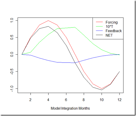
To me, Spencer’s model makes sense for illustrating his simple first point (that unknown cloud forcings could cause a misdiagnosis of the climate sensitivity).  My reproduction of his first figure using monthly steps is available here:

I don’t believe this point is in dispute — the only dispute is whether it is actually relevant here (that is, whether there exist unknown radiative forcings over the period).

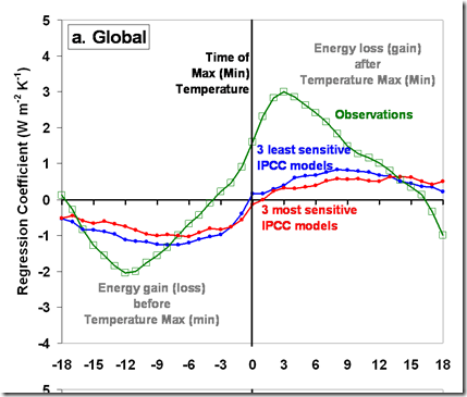
For SB’s point number two, things are not nearly as clear-cut.  I find the differences interesting, but as we’ll see later, I think figure 3 (shown below) actually undermines SB’s later point.  And as the Trenberth and Fusullo post at Real Climate points out, it is important to see to what degree the differences are the result of dataset and GCM choices.  On the other hand, adding the error bounds the way that TF does could also be misleading…what we essentially care about here is the amplitude of the variations in the lag regression plots, and so if all of the model runs have essentially the same shape but are merely shifted up or down the y-axis, it gives the impression of more uncertainty regarding the "shape" than actually exists.  The bottom plot in the TF post, which uses all models, shows so much uncertainty that it is hard to find observations that wouldn’t fit inside it.

 

The weakest part of the SB10 paper to me is point number three.  Yes, the simple model matches up well with observations, as they highlight in figure 4, and which I have attempted to reproduce below:

However, note the shape of the non-radiative forcings line, and then compare it to those lines of the climate models from SB figure 3 above.

To make the case that the climate models are off because they assume variations are not radiatively forced (in the 21st century), you would expect the climate model lines to look like the non radiatively forced line in figure 3.  Of course, the plot also uses runs from the 20th century, which includes periods where the GCM variations were largely radiatively forced, so the result is somewhat muddled.  Nonetheless, because the GCMs don’t match the non-radiative forcing line, and because they have a shape that is at least somewhat more similar to the observations than that line, it suggests that the simple model  might be missing something in this lead-lag relationship that IS present in the GCMs. That brings it to the main issue that others have raised — are there any other physically reasonable models (e.g. those that include ENSO) that can reproduce the observations?  My understanding is that Dessler 2011 focuses on whether GCMs are up to the task.

Now, with respect to the SB model and tuning, the equation seems pretty straight-forward, but with 3 major choices: 1) the depth of the ocean mixed layer, which determines heat capacity, 2) the choice of lambda (the feedback response), and 3) the choice of noise models for both the radiatively and non-radiative forcings.  The figure below shows the 70% radiatively forcing, but with lambda and the ocean layer depth changed:

At first glance the tuning doesn’t seem to be much of an issue.  The choice of ocean layer depth does not strongly affect the amplitude, whereas the sensitivity does…which is the point of the exercise.  SB are trying to show that those models with high sensitivity (lambda=1) yield the flatter lines in the regression, whereas those with low sensitivity (lambda=3) get more amplitude, and more in synch with the observations.  This perhaps explains why SB stratified GCMs in terms of climate sensitivity in their lag regression chart.  However, as shown in the TF post, the GCMs don’t necessarily break down that way. 

If the "simple model" with no radiative forcings could simulate the lagged signature of GCMs in the early 21st century, I think SB11 would have a much stronger case.  As it is, the evidence presented in the paper leaves one wondering if there are other models with non-radiatively forced ENSO variations that can also explain the lagged signature. 

However, just because I don’t find SB point #3 conclusive does not mean I necessarily agree with TF’s point #3.  That clouds respond to ENSO does not mean they can’t result in the type of misdiagnosis that SB refers to, as I explained in a comment at the Air Vent:

Consider the hypothetical scenario where winds associated with El Nino blow clouds in a specific region from over an area of low surface albedo to one of high surface albedo, thus creating a downward positive flux anomaly of X over what we would expect otherwise. Now, at the same time a global temperature increase, dT, has occured due to El Nino, causing a radiative feedback response of Y.

What we are trying to determine is the radiative response to the temperature increase, or Y/dT. But we only have the TOA flux measurement, which, since X and Y are in opposite directions, will be equal to TOA = Y – X. So obviously the (Y-X)/dT will be an underestimate, depending on the size of X.

Now, you can label X whatever you want, as it may be driven by ENSO. But X is not a response to the temperature increase of ENSO (which is what we care about WRT CO2 sensitivity), and causes an underestimate of the actual response to temperature if it is unknown or ignored.

This point seems to be missed amid all the arguments over the definitions of "forcing" or "feedback".  And yet, if this “raditively forced” portion from clouds is indeed tiny, it won’t make much of a difference.  From what I gather, Dessler 2011 dives deeper into the particular analysis of what percentage of the variation is radiatively forced.  I’m looking forward to seeing what comes out there, hopefully in another post.

As always, any comments explaining what I have wrong here are appreciated.