Radiative kernels, and more on the surface vs. atmospheric temperature feedback problem

Scripts and data for this post are available here.

CERES observation are available here.

 

CERES water vapor and cloud variables

To continue with the last post, we already know that the bulk of the temperature feedback comes from the atmosphere, not the surface.  I thus want to take a quick look here at CERES observations associated with water vapor (total precipitable water) and clouds (area fraction and optical depth) to see whether these too can be better explained using atmospheric temperatures.  A quick look at the anomalies for March 2000 through February 2010:

One thing we’ll have to watch out for in calculating our correlations is the strong temporal trend associated with the cloud optical depth.  Here is a graph of simple correlations calculated between the temperature sets and the CERES variables shown above:

From this, cloud area fraction clearly shows a better correlation with the atmospheric temperatures than the others.  However, due to the strong trend in optical depth it is not as clear cut, and the auto-correlation in total precipitable water makes it difficult to tell the best temperature index, so we’ll look at the first order differences:

 

There is not a super high correlation with any of these, but to the degree that it is there, clearly the UAH and RSS datasets are the highest. 

 

Radiative Kernels

I’ve also calculated the flux contributions of each type of feedback using radiative kernels.  This is a process I started a while back, prior to looking at this particular aspect, and is responsible for creating the largest R script I’ve ever written.  A more in-depth description (using model data) is available here, and a helpful guide here.  The basic idea is that a model is used to calculate ahead of time radiative kernels (such as those I used from Karen Shell ), which describe what each climate variable (temperature, specific humidity, albedo, etc) contributes to the TOA flux at each grid point.  These can be 2D (only lat and lon) kernels such as surface temperature and albedo, or 3D (water vapor, atmospheric temperature), which include an altitude coordinate described by the pressure level.  But these models do NOT calculate how much those variables actually change with respect to time/temperature.  For that, taking a page from the Dessler10 paper, I use the ERA interim reanalysis data as "observations", and multiple the anomalies of the climate variables by the kernels.  We are deviating a bit from true observations here, and personally I think the reanalysis data at individual grid points might be more suspect than the kernels, so make of it what you will.  

The ultimate result is the "GlobalFluxContributions" text file included.  To run the script, you’ll need to first download the ERA-interim data for BOTH the surface (temperature and albedo) and the atmosphere (relative humidity, temperature, specific humidity) at the pressure levels from 100 to 1000 described in the kernel guide above, and then rename them to match the two early references in the script.  You’ll also need to download the Shell kernels linked to above.  One thing I should also mention is that when integrating the vertical component of the kernels, they are given in units of 100 hPa. 

Anyhow, here is a graph of the flux contributions in time:

Clearly, the feedback that comes from the atmosphere in response to temperature is much larger than that from the surface.  One thing to notice is that the albedo line seems flat.  As I mentioned in my previous ERA post, this is because the ERA values for surface albedo only seem to have an annual cycle, and do not provide any interannual differences.  This is something we’ll need to keep in mind when calculating the cloud radiative forcing later.  For now, however, we can take a look at estimates of the water vapor and temperature feedbacks using the different temperature indices. 

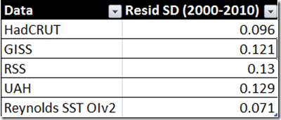
First, a mention of the variance issue mentioned by TTCA.  The following is a table of the standard deviation of the residuals of a linear regression against time:

From here on out, I’ll show the "variance normalized" calculations for feedback, where I assume the standard deviation for some "actual" surface temperature is 0.11, in the middle of the HadCRUT and GISS values.  Note that this choice DOES affect what we determine to be our actual feedback values, but is not crucial when comparing the magnitude of the feedbacks of one temperature index against another. 

For water vapor feedbacks, we get the following table:

Interestingly, using the normal surface temperatures gives both a worse correlation AND a slight underestimate of the positive feedback, even when normalized.  This, however, should not be particularly surprising, given the stronger correlation we saw above between water vapor and atmospheric temperatures. 

For the temperature feedback, once again we get a better correlation and larger estimate using the atmospheric temperatures:

However, it’s important to note that the temperature response is directly related to the temperature observations used (in this case ERA-interim), so we’re more likely to get a higher correlation based on how close the ERA observations match the other indices.  And yet, assuming that the ERA-interim reanalysis does provide realistic atmospheric observations, we see that using surface temperatures WILL underestimate the temperature response / lapse rate feedback.

To me, the issues of underestimating feedbacks by using surface temperatures seems pretty clear cut, and that whatever other problems with the simple energy balance model, using atmospheric (TLT) temps seems a step in the right direction. 

Relationship between SST and Atmospheric Temperatures, and how this affects feedback estimates

In my previous attempts to calculate feedbacks, I’ve found that typically it is the satellite temperature indices (the lower troposphere temperatures) that give the highest correlation.  There are some good reasons to think that this should be the case – for example, I’ve been working with the radiative kernels recently, and if I recall correctly some 85% of the temperature feedback response comes from the layers of the atmosphere rather than the surface.

In a recent discussion at the Air Vent, TTCA brings up an interesting point.  Basically, if the bulk of the feedback response is due to atmospheric temperature changes, then the regressions must be performed against those.  The “regression” method I’m referring to here is simply that originally pioneered by FG06 and discussed more here.  Of course, if the surface temperature variations and atmospheric temperature variations are close to one another in time, then the feedback response will be near instantaneous with the surface temperatures as well, and we should be fine.  I’ve decided to take a closer look within this post.

My script and data are available here.  The script is sort of a hodge podge of stuff, as is the post itself.

First, a quick look at the different temperature series anomalies (relative to the 2000-2010 baseline):

Now here’s a look at the correlations (r^2 values) between the various indices:

As should be clear, the satellite temperatures (UAH and RSS) correlate very well with one another, and the surface temperatures (GISS and HadCRUT) also show fairly strong correlation.  Clearly, the same “types” (surface vs. LTT) of temperatures correlate better with each other than with those of the other type.  This makes sense, but as we’ll see, one reason is because 70% of the surface is the sea surface, and atmospheric temperatures actually lag sea surface temperatures by 1-2 months.

The two SST indices I’ll be using here are HadSST2 (from CRU website) and Reynolds (I believe this is the satellite data used for GISS, and I got it from Climate Explorer):

And here is how they correlate at different lag times with the atmospheric temperatures:

Clearly, the 0 lag time does not correlate as well with atmospheric temperatures as other lag times, which suggests that the atmospheric temperatures respond to sea surface temperatures a few months later, which in turn means that using instantaneous surface temperatures to estimate feedbacks is going to decorrelate our results even further.

First, a quick look at our feedback estimate using RSS LTT.  Here I am using the CERES NET TOA flux observations (N) from my cloud feedback posts, and am estimating the forcing (Q) as simply a linear change from 0 to 0.25 W/m^2 to represent the GHG increase over the period (same estimate used in Dessler10).

This 2.93 slope (W/m^2/K) feedback corresponds to a sensitivity of around ~1.3 C per doubling of CO2.  Now, what happens if we simply use sea surface temperature (Reynolds in this case)?

We get no correlation, leading to a near-zero estimate the climate feedback and thus an extremely high climate sensitivity.  But if we use the SST anomaly from two months earlier (the approximate amount of time for the temperature changes to dominate the lower troposphere), it is quite a different story:

A much better correlation (although not great), and once again a higher estimate of feedback.  Obviously the r^2 is still not as high as either of the satellite indices, but this is to be expected if atmospheric temperatures are affected by more than simply the previous months’ SST.

Anyhow, here are the results of my runs:

Note that this does not deal with the issues from Spencer and Braswell (2010 or 2011) and Lindzen and Choi (2011) regarding forcings confounding the signal.  In this case, we’re looking at a lagged time to calculate the feedback simply because that’s when the feedback will be occurring, due to the lag in atmospheric temperature response to sea surface changes.

CERES and the SW Cloud feedback

I have a guest post up at Lucia’s going over some of my results with respect to the Dessler10 paper discussed here previously.

Surface Temperature and Albedo from ERA-interim reanalysis

This post is just a quick update on my first foray into the ERA-interim reanalysis data, in preparation for some work using the radiative kernels.  The free data that I’m using is available  at http://data-portal.ecmwf.int/data/d/interim_moda/levtype=sfc/, as long as you register.

Basically, to do a quick sanity check I was going to calculate the feedback for the easier 2D monthly parameters – skin temperature and albedo (both available at the above link).  I believe I’ll actually need to use the daily data to calculate monthly clear-sky vs. all-sky averages for these, but the monthly is a lot less data to work with while I download the other data.  The script and data available here simply read the downloaded data and performs a global spatial average.

For skin temperature the data looks good.  It matches the reanalysis temperature graph shown in figure 1C of Dessler10 (see previous post) very closely (note that my picture below is Jan 2000-Dec 2010):

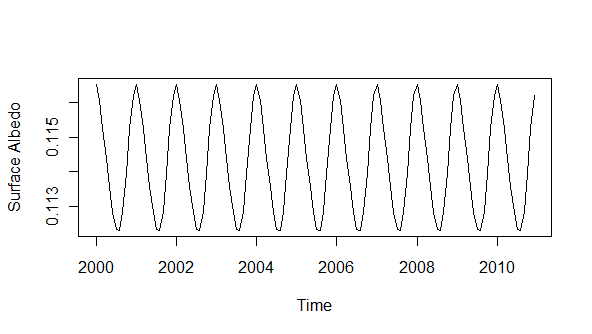
I used the same spatial average on the gridded surface albedo data per month.  Technically, this average isn’t showing the true amount of surface reflectivity; because the effect of a particular cell on shortwave flux per month will depend on its latitude (e.g. arctic albedo is going to have a much greater impact in January than in June).  However, this should give us a general idea about the albedo data:

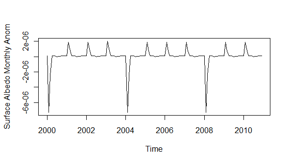
So far it looks okay, but when we remove the seasonal cycle it begins to look odd:

I’m not sure what’s going on here…it may be that albedo is estimated in such a way that it doesn’t really capture year-to-year variations.  If that’s the case, however, if will not likely be much use in calculating the feedback, nor as an input into calculating changes in clear-sky shortwave flux.  I’ll need to look into this further.