Note that by “pause in global warming” I am specifically referring to a near-halt in the underlying low-frequency signal of surface temperatures (not ocean heat content), a signal not influenced by the typical “exogenous factors” of ENSO, volcanoes, or solar activity. This has been recently attempted in Foster and Rahmstorf (2011), from which they conclude that from the “removal” of these three factors via multiple regression they have “isolat[ed] the global warming signal” and that “there is no indication of any slowdown or acceleration of global warming, beyond the variability induced by these known natural factors.” Rahmstorf et al. (2012) proceeds to compare this adjusted temperature evolution to model projections, which I think is particularly dangerous if what you get after this multiple regression approach is not the underlying signal.
Another title for this post could be, “does the multiple regression approach actually reveal the underlying signal”? Or, without spoiling too much, “is the Pinatubo recovery still contributing to the surface temperature trend?” I attempt to test this using two scenarios from a simple energy balance model, with script available here. The model is of the form ( the discrete unit of t is a month):
Which is basically the same as my previous energy balance model, except that because of the multi-decade span I have included an ocean diffusion term, which just transfers 50% of the mean TOA radiative imbalance of the year to below the mixed layer, and I’ve separated out V as the flux into the mixed layer from deeper ocean to distinguish it from a radiative forcing. It is radiatively forced by a linear “anthropogenic component”, volcanic activity, and solar activity. Variation is also induced via ENSO, and, in the case of scenario 2, a 60-year oscillation, represented by a heat flux from the lower ocean into the mixed layer. Since we will force this model using the same datasets/indices that we use to remove the influence, and we don’t introduce any other noise, I consider this a best-case scenario for the multiple regression approach.
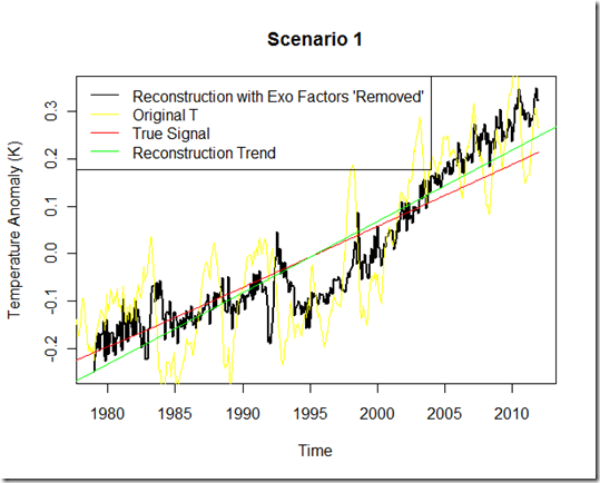
First, we have scenario 1. This has only the three “exogenous” factors and the linear anthropogenic forcing. The red line represents the global warming ”signal”…that is, the model run without the additional three factors. It starts in 1955, and thus takes a bit of time to react due to the ocean terms, but as you can see from 1979 on the “signal” is pretty much a straight line.
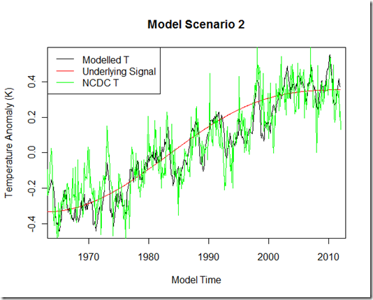
Next is scenario 2. Here again, I have included all the factors from scenario one, but I have also include a 60-yr oscillation on top of the anthropogenic forcing for the underlying low-frequency signal, which basically increases the warming trend from 1980-1995, but counteracts much of the anthropogenic forcing from 2000 to present to produce a virtual “pause”. I have included NCDC temperature anomalies to show that the modeled temperature result is pretty realistic, although with the amount of tunable parameters here (mixed layer heat capacity, ocean diffusion, radiative restoration strength) I will not be patting myself on the back for the match.
Next, I use the output from the modeled temperature and run the multiple regressions similar to the FR11 method (I do not include a Fourier series as the model contains no annual cycle). Ideally, if this method were perfect, I should be able to recover the red signal from the black.
First, we have scenario 1. For the solar and volcanic lags and “influence”, I found largely different fits when using the modeled T than FR11 found when using actual temperatures. Perhaps this is a sign that a more realistic model would yield better results for the multiple regressions, although I ‘m not sure how using a model with more complexities introduced would make it easier to pick out the influence of the different components.
The original modeled T is in yellow, whereas the new reconstructed/adjusted temperature set, with the exogenous factors “removed”, is in black. Here, we see a reduction in the variability from yellow to black, but the green line representing the slope from this reconstruction has actually increased and is greater than the true “red” signal. As such, I’m not sure the trend of black “adjusted temperatures” better represents the true signal (red) at all!
But the real test is scenario 2. Here we have an actual pause in the underlying signal “red”, and we would hope that the multiple regression method, having removed exogenous influences, would still leave that true signal intact.
As you can see, this approach yields an extremely poor “reconstruction”. One might even conclude that there was little slowdown in the warming since 2000 (trend of .178 K/decade in the reconstruction) if looking at this result, despite the fact that the true signal shows a near-halt over this period (trend of 0.037 K/decade)!
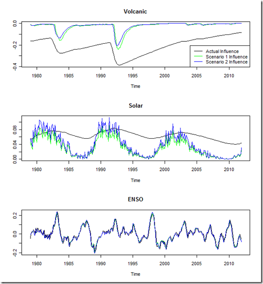
So, where did this multiple regression approach go wrong? We can diagnose this by comparing the influence determined from each regression to the actual influence in my energy balance model (determined by running the model with only that component).
First, I will note that the influence of ENSO is diagnosed extremely well. This is no doubt due to using the same index with no noise for both the forcing and determining the influence, while also noting the high-frequency and relatively high magnitude of the influence. A more complex model, or the real-world, would not likely lead to such results, but remember we’re looking at a near “best case” scenario here.
Second, we see that the solar influence is largely over-estimated. As I’ve indicated before, I think that it is hard to pick out the solar signal among the noisy data, and so given the slow-down in surface temperatures corresponding with a recent dip in solar activity, a regression model might conclude that this has a bigger impact than it actually does.
However, the biggest error here comes from an underestimate of the volcanic influence. Whereas the regression “removal” essentially sees the influence of the exogenous factor end after the forcing ends (plus whatever lag is diagnosed), the energy balance model used here shows a continuing influence through the last decade as part of the recovery. In fact, this in itself contributes about a 0.1K/dec trend to the most recent decade in the model!
Personally, I am not aware of any studies suggesting that recovery from the Pinatubo eruption might still be contributing a positive trend in 21st century temperatures. The question that arises, then, is whether this effect is just an artifact of my unrealistic model? Unfortunately, not many CMIP5 groups performed a historical, volcanic-only simulation, and the one I looked at only goes through 2005. Furthermore, the volcanic-only forcing simulations still include internal dynamics such as ENSO, so it is not that easy to isolate. Nevertheless, here is what I found for the GFDL-ESM2M run (script here):
I would say the results here are still ambiguous. The red represents a Lowess smooth, and that at least tentatively suggests an increasing trend from 2000 to present from the Pinatubo recovery, if we were to assume that that peak around 2000 and dip in 2002 were internal ENSO dynamics. Sadly, there are no more volcanic-only runs in the CMIP5 archive for this model to test that idea. There are a couple other models in the archive that have multiple runs for this, I will see if they reveal anything extra. I would also like to test the multiple regression method with different types of noise added to see how that impacts the performance as well.
Conclusions
From what I can tell, in this case, the multiple regression approach used by Foster and Rahmstorf (2011) [and Lean and Rind (2008), although I haven’t investigated the specifics of that paper] can produce misleading results, even failing to recognize a pause in the underlying signal. In those cases, the “reconstruction” can be a worse representation of the true signal than the original, unadjusted results, and should not be used to test projections. Of course, in this particular case, much of it seems to stem from a lingering effect of the Pinatubo recovery into the 21st century, which I am currently skeptical exists in the real world.


