Comment on “The phase relation between atmospheric carbon dioxide and global temperature”

This may seem a bit trivial, but since Humlum, Stordahl, and Solheim (2012)) was published in Global and Planetary Change, I thought it may be worth addressing, particularly while I still have access to these paywall articles.  From the “highlights” on that link, I will note the following points:

► The overall global temperature change sequence of events appears to be from 1) the ocean surface to 2) the land surface to 3) the lower troposphere. ►Changes in global atmospheric CO₂ are lagging about 11–12 months behind changes in global sea surface temperature. ► Changes in global atmospheric CO₂ are lagging 9.5-10 months behind changes in global air surface temperature. ► Changes in global atmospheric CO₂ are lagging about 9 months behind changes in global lower troposphere temperature. ► Changes in ocean temperatures appear to explain a substantial part of the observed changes in atmospheric CO₂ since January 1980. ► CO₂ released from use of fossil fuels have little influence on the observed changes in the amount of atmospheric CO₂, and changes in atmospheric CO₂ are not tracking changes in human emissions. 

My bold.  Essentially, the method in HSS12 is to compare the “DIFF12” values for each time series – that is, for each month they find the difference between the last 12 months and the 12 preceding months.  In general, they find that the fluctuations in DIFF12 of temperatures lead the fluctuations in DIFF12 of atmospheric CO2, and then conclude:

In general, we find that changes in atmospheric CO2 are lagging behind changes in any of the five different  temperature records considered. The typical lag is 9.5-12 months for surface temperatures and about 9 months for lower troposphere temperatures, suggesting a temperature sequence of events from the surface to the lower troposphere.

As cause always must precede effect, this observation demonstrates that modern changes in temperatures are generally not induced by changes in atmospheric CO2. Indeed, the sequence of events is seen to be the opposite: temperature changes are taking place before the corresponding CO2 changes occur.

In case one may mistake this to mean “temperature changes on a short-term scale”, they discuss later:

A main control on atmospheric CO2 appears to be the ocean surface temperature, and it remains a possibility that a significant part of the overall increase of atmospheric CO2 since at least 1958 (start of Mauna Loa observations) simply reflects the gradual warming of the oceans, as a result of the prolonged period of high solar activity since 1920 (Solanki et al. 2004).

For me, the easiest way to prove that the conclusions don’t follow from a particular method is to use a simple model where we know the actual causes and parameters, and then see if using the particular method will accurately diagnose the “cause.” 

Here, I’ll dust off that old one-box energy balance model.  Script is available here.  Some key aspects of this demo:

• I’ve set the increase in CO2 due to anthropogenic emissions to increase at a nearly linear rate of about 2 ppm / year, with some slight curvature for realism.
• I’ve included ENSO variations for temperature changes, using the actual Nino34 index.
• I’ve set the atmospheric CO2 value to respond slightly to temperature after 11 months.

Running the “simulation” yields the following temperature response:

 

And here is the annual atmospheric CO2 for the run:

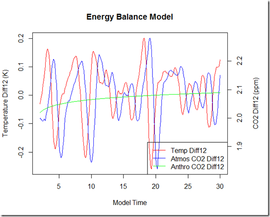
As you can see, that annual CO2 seems to vary little from temperature changes. But what happens when we use the DIFF12 method from HSS12?

 

Well, according to HSS12, this graph would imply that most of the CO2 increase over the model run must be due to surface/ocean warming (and not the other way around), since temperature diffs clearly lead those CO2 DIFF changes by 11 months!  Furthermore, anthropogenic CO2 would appear to have almost no effect on total atmospheric CO2!  Of course, there’s one huge problem with these conclusions: we know that they are wrong, because we set the parameters for the model.  In fact, we can calculate precisely the percent of the atmospheric CO2 increase that was caused by surface warming by subtracting the “resulting” atmospheric CO2 from the anthropogenic CO2: 0.33 ppm out of 62.2 ppm, or 0.5%.  In other words, 99.5% of the CO2 increase in this model run is the result of the programmed anthropogenic emissions, despite what the DIFF12 chart would appear to show.

Clearly, the HSS12 “DIFF12” method is not able to diagnose the long-term cause vs. effect.  Rather, it is quite easy for a small CO2 response to temperature, particularly one which will have no long-term impact, to create results in the DIFF12 graphs that make them appear (incorrectly) to provide great explanative power.  In other words, the method chosen in the paper does not support its conclusions.

So, does anybody with an academic grant for page fees want to take lead author on the reply for some easy publication credit? :)  

Sensitivity of the water vapor feedback to locations of SST trends

With a new computer that has the necessary disk space and memory, I was finally able to do some of the analysis I had talked about doing in the previous post, and the preliminary results seem quite interesting.  To recap, I wanted to see what effect the discrepancy in the rates of sea surface warming at different latitudes would have on the TOA radiation budget that could specifically be attributed to water vapor.  This was originally to check out Dr. Pielke Sr.’s  hypothesis that perhaps the different rates of evaporation in these areas would have an impact on the water vapor feedback.

 

Data and Methods

Here, I use the same 5 CMIP5 historical runs from the GFDL CM2.1 model as I did in that last post, in particular the specific humidity and surface air temperature values.  I estimated the TOA radiative impact specifically attributed to water vapor for each month by using the longwave water vapor radiative kernel  derived from GFDL CM2.1.  I then compared this against the 3 GFDL HIRAM C180 AMIP runs available on the GFDL data portal, again converting specific humidity to the corresponding radiative anomaly.  Since the primary difference between the CMIP and AMIP runs is that the AMIP runs have the atmospheric model responding to actual sea surface temperature observations, if we assume that the atmospheric model in GFDL’s CM2.1 is very similar to GFDL’s HIRAM C180, we are thus essentially able to isolate the different water vapor responses specifically to the discrepancy in the location of SST trends.    The code and intermediate data for this post can be found here.

 

Results

In the figure above you can see the trend in the outgoing longwave radiation (OLR) over time in the coupled vs. atmosphere-only model runs.  The lower the OLR anomaly, the more heat that is "trapped" due to water vapor.  It is interesting to note that the AMIP runs, bounded as they are by actual SST observations, see a trend that has a much smaller magnitude than the fully coupled models (and, unsurprisingly, the runs show much less variation).  Clearly the discrepancy in SST trends has had a large impact on the TOA balance, at least with respect to water vapor.  However, if we’re estimating a global factor for the water vapor feedback, this in itself would not necessarily indicate an overestimation of the feedback (dR/dT) in the CM2.1 coupled model, since perhaps the denominator for the coupled model (the temperature trend) has been overestimated just as much as dR (one may argue that an overestimation in temperature trend could indirectly indicate an overestimate of some positive feedback, but it is by no means straight-foward).   

The figure below shows the temperature trend in the coupled runs vs. GISS.  I should mention that it is my understanding that the long term water vapor feedback will be primarily driven by ocean temperatures, rather than including land surface air temperatures.  However, given that feedbacks and sensitivity estimates are typically calculated with respect to surface air temperature, I’ve framed the results in this way to be able to make meaningful comparisons to other results.  As we can see, the trends tend to be higher in the coupled runs, but the difference in trends is not as drastic as in the OLR anomalies.

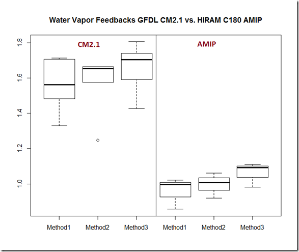
Additionally, there are are few different ways we might calculate the feedback ratio, dR/dT.  Soden and Held (2006) take the mean from the last 10 years and subtract the mean from the first 10 years when calculating the feedback from models, but they had 110 years to work with; since we only have 28 years here, I’ve employed a similar method (method #2 in the figure below) using the mean from the last 5 years (2004-2008) and the first 5 years (1981-1985).  Another method I’ve employed (method #1), in order to use all years, is the ratio of linear trends in the wv-induced OLR changes and temperature changes, or (dR/dt) / (dT/dt) (such a method is used, for example, when determining trend amplification in land vs. ocean vs. lower troposphere).  These methods, I believe, are more likely to highlight the long-term (climate scale) radiative variable response relevant to climate sensitivity.

The final method (method #3) I show is regressing R_wv (yearly anomalies) directly against temperatures.  This method has been used in several papers where the satellite observations are limited (to ~10 years).  However, in this approach, you tend to be measuring the response to ENSO-induced interannual variability, unless the trends are strong enough to negate this…and as I’ve discussed before, there appears to be little evidence to suggest that the global radiative response to ENSO-induced temperature changes correlates well with the long-term response, and it certainly doesn’t in most models.   

And thus we have a boxplot of the estimated water vapor feedback:

    

Conclusions and Limitations

A simple glance would suggest that the water vapor feedback is significantly lower (~40%) in those runs bounded by SST observations than the coupled runs, which would have potentially large impact on the estimated sensitivity (for example, all else being equal and assuming a an average water vapor feedback of 1.8 W/m^2/K in models, this sort of reduction in the WV feedback would lower the climate sensitivity estimate from 3.0 K to 1.9 K).  However, there are a  couple of large caveats here, the first of which is whether a similar warming pattern of the sea surface (lower in the tropics) would be expected with the continual increase in CO2, or whether some sort of natural variability is impacting this pattern.  This goes for land vs. SST as well, where it appears the discrepancy between the SST and land rates is greater in observations than in the coupled model.  Additionally, it is quite possible that some of the lessening of the positive water vapor feedback may be counteracted by a decrease in the strength of the negative lapse rate feedback which could mitigate the effect on overall sensitivity.

Another thing that should raise some question marks is that all of the methods above during this time period seem to underestimate the 100 year water vapor feedback for GFDL CM2.1, at least according to Soden and Held (2006), where it is listed as 1.97 W/m^2/K.  Also, the all-sky radiative kernel should not be entirely relied upon, as it is based on the models that do not accurately represent the cloud distribution (see errors in all-sky outgoing radiation).  One may also wonder why we don’t use available reanalysis.  Apart from the fact that we want to isolate the differences simply to water vapor concentrations resulting from observed sea surface temperatures, reanalysis products have also been shown to be inadequate for the task of reproducing long-term trends in water vapor [John et al., 2009 ; Serreze et al., 2012].          

So, with regards to the original question about whether the discrepancy in the spatial distribution of sea surface temperature trends may affect the water vapor feedback specifically because of the different rates of evaporation, the last two posts at least provide some support for the hypothesis.  I could not say evaporation is the key here for sure, but neither do I see any evidence to dispute it.

I am a bit curious as to whether this method has been employed before (that is, combining AMIP models with radiative kernels for comparison against coupled runs for feedback analysis), as it seems straightforward and could provide a more extended period of analysis than is available in the satellite record.  It seems like it could be an interesting avenue to explore.