ERBE, Pinatubo, and Climate Sensitivity

In Forster and Gregory 2006, the authors pioneered a fairly straight-forward  method of estimating climate sensitivity based on the top-of-atmosphere flux imbalance, the net forcing, and the corresponding surface temperature changes.  Somewhat recently, Roy Spencer used basically the same method to estimate sensitivity from the Pinatubo eruption, and got different results from what they got in the paper.  I was curious about the difference, particularly since  Eli Rabbet brought up what seemed to me to be a valid objection: “Still, in this case you have to handle the fact that using the MSU you are making the measurement in the middle of the system and not at the bottom.”  I wanted to see what would happen if I used surface temperatures instead of TLT.  I also wanted to try and reproduce the analysis in a script and using available on-line data so that it might be obvious if a mistake was made.

Part 1: Running on Annual Data 1985-1996

After having some difficulty running the reading software associated with the raw ERBE data files from ASDC, and worried I would have to perform the global averaging and adjustments myself that were mentioned in the paper, I was happy to eventually stumble upon the page with the revised data maintained by Dr. Wong.  I use the ERBE_S10N_WFOV_ERBS_Edition3_Rev1 72-day near global means for the TOA flux at this page.

For the forcings, I use GISS’s  estimated WMGHG and Stratospheric Aerosol forcings used in the models.

For surface temperatures I use GISTemp and HadCRUT values.  The script for this part can be found here.

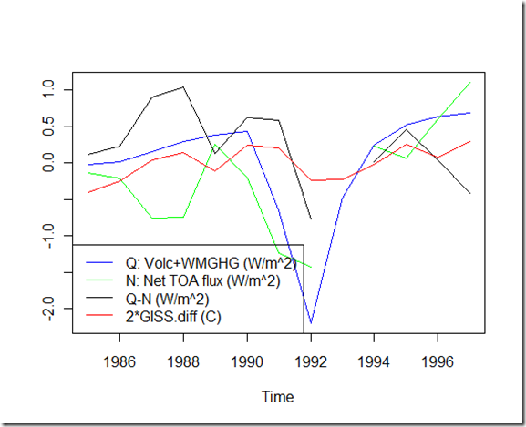
Here’s a quick look at the different factors, which should be comparable to the middle-right graph of figure 2 in the FG06.  The main difference here  is that I include 1997 (which I’ll mention later) in both the graph and the baseline, so some of the lines are slightly shifted vertically:

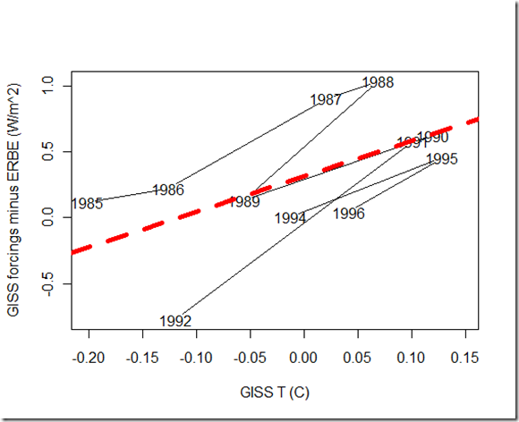
Now, for the actual regression on the annual means against both GISS and HadCRUT:

For GISS, I get a value of Y that is 2.70 W/m^2K (1.4 degrees C per CO2 doubling), with a 2.5%-97.% confidence interval of [-.052, 5.44], and a correlation = .59.  The chart matches up pretty well with the middle-right in figure 3 of the paper, although they get a Y of 2.32 with a correlation = 0.66.  

For HadCRUT it is similar, yielding a Y of 2.76 W/m^2K, a confidence interval of [-.562, 6.08], and a correlation = .53.  In the FG06 paper they get Y=2.5, and a correlation of .54.

I think the slight differences between my results and those of the FG06 paper in this case might be related to the newer datasets (after all, the paper was from 5 years ago), but I’m not 100% sure.

One thing worth noting is that 1993 and 1997 have been excluded from the analysis, per FG06.  1993 is missing several 72-day cycles of data for ERBE WFOV, so this makes sense.  I’m a bit confused about the reason for excluding 1997:

However, the two surface temperature time series shown give quite different changes between 1996 and 1997. As our approach is dependant on stable time series of robust data, 1997 was excluded from subsequent analysis.

With both GISTemp and HadCRUT, adding 1997 seems to significantly hurt the fit and bring down the correlation.  Y’s drop to 1.59 and .872 respectively, with correlations dropping to .35 and .18.  So, while the year-to-year change of 1996 to 1997 might be different between GISTemp and HadCRUT, either way creates an outlier.  I’m a bit surprised that more was not made of this fact.

Nonetheless, the main focus here is on the differences in the seasonal/72-day average estimates of climate sensitivity during the Pinatubo years…

 

Part 2: Pinatubo Years 1991-1993

The main script for this part, where I use 5 measurements per year, can be found here.  The other scripts for the extra seasonal analysis can be retrieved here.

There are a couple of challenges using the multiple measurements per year versus annual averages.  First, I had to use the monthly Sato measurements for the volcanic forcing rather than the annually averaged GISS forcings.  I ignored the WMGHG forcing in this case because the magnitude of the change in WMGHG forcing over the Pinatubo years is dwarfed in comparison to the variability in the volcanic forcing. 

Second, the 72-day ERBE data for near global means needs to be used due to satellite sampling issues, which means 5 measurements per year.  With only monthly volcanic and surface temperature measurements, this meant interpolating some values using spline.  Going from frequency 12->5 by the method in the script seems to work pretty well for most cases in my synthetic data tests.

Anyhow, here are graphs of the results for GISSTemp and HadCRUT:

    

Both of these values seem to match the low climate sensitivity that Dr. Spencer got in his analysis, although the correlations aren’t quite as good.  The Y values are higher than those estimated in the FG06 paper, which had (2.1 W/m^2K and 2.9), although those correlations were closer to mine if you take into account the 12 data points used here vs. the 8 in the paper.

So, at first glance it seems that using surface temperatures does in fact yield a similar results to the TLT temperatures.  This means that the differences between Dr. Spencer’s analysis and those in FG06 cannot simply be attributed to that. 

One obvious difference is that FG06 uses seasonal values (frequency=4) vs the 72-day averages.  I’m not entirely sure at this point how the authors determined the ERBE seasonal values, but I tried two different methods:

First, I simply averaged the monthly values for the ERBE data.  This, of course, does not necessarily eliminate the sampling errors, and I believe Lindzen and Choi (2009) was criticized for doing it.  It thus resulted is a strangely high value for Y of 14 W/m^2K (0.27 C for a doubling of CO2) with a correlation of 0.72.

The second method was to use spline to convert the 72-day averages to seasonal averages for the ERBE data.  Going from 5->4 frequency seems to introduce more error  than 12->5, which is why I didn’t do it for my primary method.  The result it a Y value of 5.44 with a correlation of 0.74. 

So, neither of these conversions to seasonal data seemed to reproduce the higher sensitivity in the FG06 results for the Pinatubo years.  It will remain a mystery for now at least, but I’ll do some more digging (and perhaps drop the authors a line) when I have more time.