The question of how much more warming is "in the pipeline" or we are "committed to", if we stopped emissions immediately, is an interesting but not quite trivial one to answer. Sure, there are GCMs that can run this scenario, but given their seeming inability to correctly reproduce the effective sensitivity relevant on these timescales (Masters, 2013) or the magnitude of the aerosol forcing (as appears to be the case in AR5 drafts), it would be nice to see how these factors influence the amount of warming we could expect under this scenario.
As part of a larger project, I have been developing some much simpler models that simulate the properties of the CMIP5 multi-model-mean under the various RCP scenarios up to the year 2100, but with the ability to enter specific values for parameters like effective sensitivity, current aerosol forcing, and emissions trajectories that have the largest impact on the warming. I thought this scenario would be an interesting test for this portion of it (you might notice my R code in this case has the distinctive feel that it has been ported from a different language).
For the first part, we need to know how the temperature responds to forcings. Obviously, one parameter we will take into account is "effective sensitivity", or rather its inverse in the form of radiative restoration strength – this is the value provided by the "user" or the model. While the radiative restoration strength is not necessarily a constant, as discussed in previous posts, we want to take a value that is relevant on the century scale. However, even if the user prescribes this value, we still need to know how fast the temperature will approach this value for a given forcing evolution. For that part, I attempted to "reverse engineer" the values for the CMIP5 multi-model mean (which is itself a hodge-podge of various runs from various models), by using 1.18 W/m^2/K for radiative restoration (3.1K Effective Sensivity), as I found in my paper, and proceeded to fit the remaining parameters based on the adjusted forcings and temperature evolution of the 4 RCP scenarios as shown in Forster et al. (2013). While a one-box model did not quite give a great fit across the various scenarios, using a 2-layer model as described in Geoffroy et al. (2013) seems to do the trick.
For the second part, we need to know the actual forcing evolution. This too requires some reverse engineering and simplifying assumptions. In this case, since we are stopping emissions immediately, those species with atmospheric lifetimes << 1 year can see their forcings drop to 0 immediately (aerosols, O3). For other species, I assumed a constant "effective atmospheric lifetime" and atmospheric fraction, again fitting these values based on the RCP scenarios. This yielded an effective lifetime of 12 years for CH4 and 185 years for CO2. Since N20 and the main contributing CFC have similarly long lifespans, I simply lumped these smaller effects in with CO2 by slightly increasing the CO2 forcing for a given concentration (again, I don’t want my "simple" model to require the user to enter 10 different emissions trajectories!).
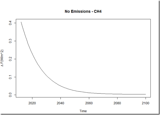
Here are the resulting forcing evolutions for the major greenhouse gases were emissions to stop today:
As you can see, due to the longer lifetime of CO2, the decrease in forcing is rather slow over time. On the other hand, methane drops off rather quickly. Contrary to the GHG forcing, we would likely see a large jump *up* in forcing from aerosols if we stopped emitting immediately…the magnitude of that jump up obviously depends on the magnitude of the current aerosol negative forcing.
Below are the temperature evolutions for different values of effective sensitivity and aerosol forcing. For effective sensitivity, I will show the value of 1.8K (as found in my paper), as well as 3.1 K (as I found for the CMIP5 models). For the aerosol forcing, I will use the values of -1.3 W/m^2 (AR4) and -0.9 W/m^2 (last draft of AR5). Note that this additional warming chart is only taking into account anthropogenic forcings…it does not include the warming or cooling influences that may come from natural forcings in the future.
As you can see, all of them have a "bump" within the next 10 years, which represents the immediate increase in forcing due to the drop-off of aerosols. After that, the temperatures begin to drop as the methane concentrations and CO2 concentrations begin to decrease. However, the magnitudes are very different! In these scenarios, choosing different values of sensitivity and aerosol forcing (from what I consider realistically possible values), can mean the difference between 0.6 K and 0.2K warming in the pipeline. To further highlight this dependence, I will show the more "extreme" values based on the edges of uncertainty of sensitivity and aerosols:


