1. Introduction
Typical energy balance methods, such as Otto et al (2013) or Masters (2014), have been frequently used for estimating equilibrium climate sensitivity (ECS) over the instrumental period. Recently, several studies have raised the possibility that these may be biased, even if one were to precisely pin down the magnitude of the aerosol forcing and the current top-of-atmosphere (TOA) energy imbalance. In particular, the net feedback or radiative restoration parameter (typically represented by lambda) may be different when calculated over the instrumental period vs. the long-term, idealized CO2-only simulations. One could partition this into two factors:
1) Inhomogenous Forcings. Certain forcings, such as aerosols, may be concentrated in higher-latitude regions, where the net feedback is smaller, thereby “cancelling out” more of the homogenous greenhouse forcing when looking only at the globally-averaged TOA imbalance. This was raised recently in the Kummer and Dessler (2014) extension of the Shindell (2014) forcing “enhancement” from TCR to ECS (although as discussed previously, the enhancements in TCR and ECS are very different).
2) Time-Varying Sensitivity. Armour et al (2013) suggest that this may result from time-invariant local feedbacks, with only the spatial warming pattern changing over time and triggering these local feedbacks in changing proportions over time.
In fact, if we take the Armour et al (2013) view, both #1 and #2 have the same root cause – the differing spatial warming pattern between the transient, instrumental warming pattern case, and the long-term idealized 2xCO2 scenarios run in the models.
2. Method
If you will recall, one of my criticisms of Shindell et al (2014) was that it did not consider the observed spatial warming pattern. Essentially, when determining forcing enhancements, it relied on the GCM output for:
a) The ratio of the localized temperature response relative to the global response (essentially the relative heat capacity of each region)
b) The spatial warming pattern in the idealized GHG scenarios
c) The spatial warming pattern over the historical/instrumental period
While a and b may need to be relied upon, it seems as though one could use the information from c during the observed instrumental period, rather than relying on something that GCMs do poorly (regional warming projections, response to aerosols, and horizontal heat transfer). Moreover, an ensemble of runs from a GCM will not be able to reproduce the exact variability seen in the single “realization” of the instrumental period. To me, it seems more likely that GCMs might be more correct and agree better on a and b than they would on c. But even if they are not, at least it is one less assumption that needs to be made regarding GCM accuracy.
By analogy, I think there is a reasonable method for determining the bias in ECS when calculated over the instrumental period. Essentially, for different GCMs, we would calculate
a) The zonal net feedback according to the GCM. We do this by first calculating the forcing for each zone using the difference in TOA imbalance for the last 25 years of the fixedSST regressions: sstClim4xCO2 – sstClim. Then, for each zone we calculate the difference in TOA balance between the abrupt4xCO2 experiment and the piControl experiment, subtract the forcing calculated in the prior step, and normalize this by the local temperature increase calculated as the difference between abrupt4xCO2 and the piControl. Note: this relies on the assumption of Armour et al (2013) that the increase in surface temperature in one region primarily affects the outgoing radiative response locally, rather than over some other area. At the end, we have an n x 1 column vector A, with n being the number of zones.
b) The spatial warming pattern over the idealized scenario from the GCM that we will use as a baseline. For example, if one were interested in how inhomogenous forcings may create a bias in energy balance estimates over the instrumental period, one might use the historicalGHG or abrupt4xCO2 scenario over a time period similar to the length of the historical period. If, on the other hand, one wanted to figure out the combined effect of those inhomogenous forcings + time-varying sensitivity, one would use the spatial warming pattern of a run that had achieved radiative equilibrium after a doubling of CO2. Regardless, we calculate an n x 1 column vector B, which consists of each of zone’s temperature change, normalized by the global temperature change.
c) The observed spatial warming pattern. Similar to the step above, we calculate an n x 1 column vector C, which consists of each zone’s observed temperature change over the instrumental period, normalized by the total global temperature change.
Finally, we can then calculate what the expected bias in net feedback calculated over the instrumental period will be, according to each model, using the following equation:
Eq. 1
Where the function “weight” simply multiplies each element in the vector by its area fraction of the globe.
3. Example with GFDL-CM3
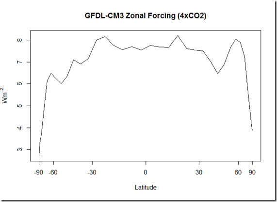
First, here is the fixed-SST forcing calculation:
One thing of interest here is that the global forcing actually comes out to 7.2 W/m^2 for 4xCO2, which is more in line with the typical value of 3.7 W/m^2 for a doubling of CO2, and well above what is calculated in Andrews et al (2012) using the regression technique. However, a look at figure 1 from Andrews et al (2012) highlights why:
As you can see, there is one point with a net imbalance above the intercept at 6 W/m^2 which Andrews et al (2012) takes as the forcing. Clearly, since the regression is affected greatly by the larger T points and there is significant curvature, the regression method in this case underestimates the forcing.
Moving on, here is the calculation of the zonal net feedbacks:
Interestingly, this seems to differ from the local feedbacks of the CCSM4 model used in Armour et al (2013). However, the primary difference seems to be the peak response at –60 degrees that does not appear to be present in that CCSM4 model.
Next up, here are the normalized temperature responses for the different scenarios in GFDL-CM3, along with the observations from Cowtan and Way (2014).
What is obvious in the GFDL-CM3 historical pattern is the dip in temperatures between 30 and 60 degrees in the northern hemisphere, which seems a pretty clear indication of the aerosol response in that model. In the observed historical record, this dip appears to be absent, and overall the observed warming pattern seems much more similar to the historicalGHG and abrupt4xCO2 scenarios than the historical scenario, apart from the lack of Arctic warming
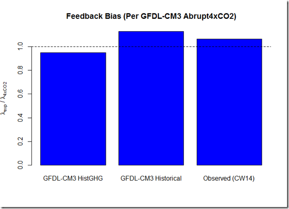
Finally, if one where to calculate the feedback bias relative to the abrupt4xCO2 scenario, we find the following ratios:
This essentially isolates the expected forcing “enhancement” bias, as it is baselined against the idealized 4xCO2 run. In this case, the above ratios are 0.95 (histGHG), 1.13 (historical), and 1.06 (observed). This suggests that if one used the historicalGHG runs to estimate ECS, there might be a slight overestimate relative to the CO2-only run, as GFDL-CM3 includes the inhomogenous ozone forcing in their histGHG runs. Were one to trust the relative strength of zonal feedbacks in GFDL-CM3, it suggests about a 6% underestimate of ECS from energy balance methods over the instrumental period due to the inhomogenous aerosol forcings. However, ideally one could use this method with a variety of GCMs to identify the expected bias among a wider array of models.
Moreover, if one were interested in the bias of “effective sensitivity” (EFS) relative to ECS, one would ideally get a longer run of GFDL-CM3 with a doubling (or quadrupling) of CO2, and see how the warming pattern ended up after it reached equilibrium. Unfortunately, I am not aware of any such output currently available for this model.
***Final note: in my calculations, I initially performed the analysis using land and ocean zonal feedbacks and temperatures separately, rather than combined into one. For GFDL-CM3, this did not seem to make much difference, and I did not readily have available separately gridded land and ocean temperatures from observations. However, I seem to recall that the response was substantially different between land and ocean in Armour et al (2013), so perhaps it a more wide-ranging survey of GCMs it would be better to separate these out again.
Does anybody else think this a promising method for leveraging historical observations in estimating the potential bias in energy balance estimates?
Code and Data
- Scripts and intermediate data for this post.
- GFDL Data Portal
- Cowtan and Way (2014) data page


