Breaking down the discrepancy between modeled and observed temperatures during the “hiatus”

 

Introduction

There are many factors that have been proposed to explain the discrepancy between observed surface air temperatures and model projections during the hiatus/pause/slowdown. One slightly humorous result is that many of the explanations used by the “Anything but CO2” (ABC) group – which argues that previous warming is caused by anything (such as solar activity, the PDO, or errors in observed temperatures) besides CO2 – are now used by the “Anything but Sensitivity” (ABS) group, which seems to argue that the difference between modeled and actual temperatures may be due to anything besides oversensitivity in CMIP5 models. And while many of these explanations likely have merit, I have not yet seen somebody try to quantify all of the various contributions together. In this post I attempt (perhaps too ambitiously) to quantify likely contributions from coverage bias in observed temperatures, El Nino Southern Oscillation (ENSO), post-2005 forcing discrepancies (volcanic, solar, anthropogenic aerosols and CO2), the Pacific Decadal Oscillation (PDO), and finally the implications for transient climate sensitivity.

Since the start of the “hiatus” is not well defined, I will consider 4 different start years, all ending in 2013. 1998 is often used because of the large El Nino that year, which minimizes the magnitude of the trend starting in that year.  On the other hand, the start of the 21^st century is sometimes considered as well. Moreover, I will use HadCRUTv4 as the temperature record (since this is the more cited to represent the hiatus), which will show a larger discrepancy at the beginning than GISS, but will also show a larger influence from the coverage bias. The general approach here is to consider that IF the CMIP5 multi-model mean (for RCP4.5) is unbiased, what percentage of the discrepancy can we attribute to the various factors? Only at the end do we look into how the model sensitivity may need to be “adjusted”. Note that each of the steps below are cumulative, building off of previous adjustments. Given that, here is the discrepancy we start with:

Start year	HadCRUT4 (K/Century)	RCP4.5 MMM (K/Century)
1998	0.44	2.27
1999	0.75	2.16
2000	0.44	2.01
2001	-0.08	1.92

 

Code and Data

My script and data for this post can all be downloaded in the zip package here. Regarding the source of all data:

· Source of “raw” temperature data is HadCRUTv4

· Coverage-bias adjusted temperature data is from Cowtan and Way (2013) hybrid with UAH

· CMIP5 multi-model mean for RCP4.5 comes from Climate Explorer

· Multivariate ENSO index (MEI) comes from NOAA by way of Climate Explorer

· Total Solar Irradiance (TSI) reconstruction comes from SORCE

· Stratospheric Aerosol Optical Thickness comes from Sato et al., (1993) by way of GISS

· CMIP5 multi-model mean for natural only comes from my previous survey

· PDO index comes from the JISAO at the University of Washington by way of Climate Explorer.

 

Step 1: Coverage Bias

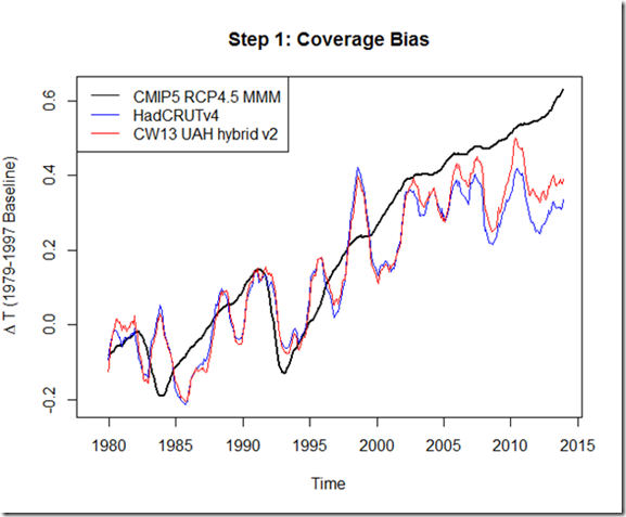
For the first step, we represent the contribution from coverage bias using the results from Cowtan and Way (2013). This is one of two options, with the other being to mask the output from models and compare it to HadCRUT4. The drawback of using CW13 is that we are potentially introducing spurious warming by extrapolating temperatures over the Arctic. The drawback of masking, however, is that if indeed the Arctic is warming faster in reality than it is in the multi-model-mean, then we are missing that contribution. Ultimately, I chose to use CW13 in this post because it is a bit easier, and because it likely represents an upper bound on the “coverage bias” contribution. I may examine the implications of using masked output in a future post.

The above graph is baselined over 1979-1997 (prior to the start of the hiatus), which highlights the discrepancy that occurs during the hiatus.

Start year	S1: HadCRUT4 Coverage Adj (CW13, K/Century)	RCP4.5 MMM (K/Century)
1998	1.10	2.27
1999	1.38	2.16
2000	1.05	2.01
2001	0.54	1.92

Step 2: ENSO Adjustment

The ENSO adjustment here is simply done using multiple linear regressions, similar to Lean and Rind (2008) or Foster and Rahmstorf (2011), except using the exponential decay fit for other forcings, as described here.  While I have noted several problems with the LR08 and FR11 approach with respect to solar and volcanic attribution, which I mention in the next step, I also found that ENSO variations are high enough frequency so as to be generally unaffected by other limitations in the structural fit of the regression model.

 

Step 3: Volcanic and Solar Forcing Updates for Multi-Model-Mean

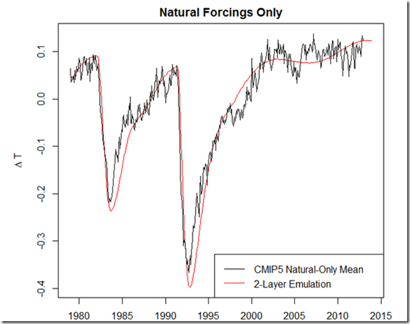
The next step in this process is a bit more challenging. We want to see to what degree updated solar and volcanic forcings would have decreased the multi-model mean trend over the hiatus period, but it is quite a task to have all the groups re-run their CMIP5 models with these updated forcings. Moreover, as I mentioned above and in previous posts (and my discussion paper), simply using linear regressions does not adequately capture the influence of solar and volcanic forcings. Instead, here I use a two-layer model (from Geoffrey et al., 2013) to serve as an emulator for the multi-model mean, fitting it to the mean of those natural-only forcing runs over the period. This is a sample of the “best fit”, which seems to adequately capture the fast response at least, even if it may be unable to capture the response over longer periods (but we only care about the updates from 2005-2013):

 

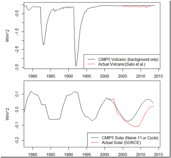
And here are the updates to the solar and volcanic forcings (updates in red). For the volcanic forcing, we have CMIP5 volcanic aerosols returning to background levels after 2005. For the solar forcing, we have CMIP5 using a naïve, recurring 11-year solar cycle, as shown here, after 2005.

The multi-model mean is then “adjusted” by the difference between our emulated volcanic and solar temperatures from the CMIP5 forcings and the observed forcings. The result is seen below:

Over the hiatus period, the effect of the updated solar and volcanic forcings reduces the multi-model mean trend by between 13% and 20%, depending on the start year.

 

Updated anthropogenic forcings?

With regards to the question of how updated greenhouse gas and aerosols forcings may have contributed to the discrepancy over the hiatus period, it is not easy to get an exact number, but based on evidence of concentrations and emissions that I’ve seen, there does not seem to be a significant deviation between the RCP4.5 scenario from 2005-2013 and what we’ve observed. This is unsurprising, as the projected trajectories for all of the RCP scenarios (2.6, 4.5, 6.0, 8.5) don’t substantially deviate until after this period.

For instance, the RCP4.5 scenario assumes the CO2 concentration goes from 376.8 ppm in 2004 to 395.6 ppm in 2013. Meanwhile, the measured annual CO2 concentration has gone from 377.5 ppm in 2004 to 396.5 ppm in 2013. By my back-of-the-envelopment calculation, this means we have actually experienced an increase in forcing of 0.002 W/m^2 more than in the RCP4.5 scenario, which is a magnitude away from being relevant here.

For aerosols, Murphy (2013) suggests little change in forcing from 2000-2012, the bulk of the hiatus period examined. Klimont et al (2013) find a reduction in global (and Chinese) sulfur dioxide emissions since 2005, compared to the steady emission used in RCP4.5 from 2005-2013, meaning that updating this forcing would actually increase the discrepancy between the MMM and observed temperatures. However, it seems safer to simply assume that mismatches between projected and actual greenhouse gas and aerosol emissions have contributed a likely maximum of 0% to the observed discrepancy over the hiatus, and it is quite possible that they have contributed a negative amount (that is, using the observed forcing would increase the discrepancy).

 

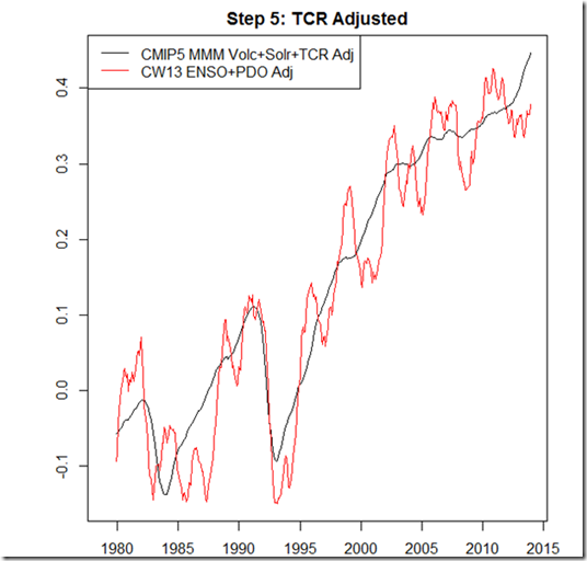
Step 4 & 5: PDO Influence and TCR Adjustment

Trying to tease out the “natural variability” influence on the hiatus is quite challenging. However, most work seems to point to the variability in the Pacific: Trenberth and Fasullo (2013) suggest the switch to the negative phase of the PDO is responsible, causing changing surface wind patterns and sequestering more heat in the deep ocean. Matthew England presents a similar argument, tying in his recent study to that of Kosaka and Xie (2013) over at Real Climate.

In general, the idea is that the phase of the PDO affects the rate of surface warming. If we assume that the PDO index properly captures the state of the PDO, and that the rate of warming is proportional to the PDO index (after some lag), we should be able to integrate the PDO index to capture the form of the influence on global temperatures. Unfortunately, because of the low frequency of this oscillation, significant aliasing may occur between the PDO and anthropogenic component if we regress this form directly against observed temperatures.

There are thus two approaches I took here. First, we can regress the remaining difference between the MMM adjusted for updated forcings and the ENSO-adjusted CW13, which should indicate how much of this residual discrepancy can be explained by the PDO. In this test, the result of the regression was insignificant – the coefficient was in the “wrong” direction (implying that the negative phase produced warming), and R^2=0.04. This is because, as Trenberth et al. (2013) note, the positive phase was in full force from 1975-1998, contributing to surface warming. But the MMM matches too well the rate of observed surface warming from 1979-1998, leaving no room for the natural contribution from the PDO.

To me, it seems that if you are going to leave room for the PDO to explain a portion of the recent hiatus, it means that models probably overestimated the anthropogenic component of the warming during that previous positive phase of the PDO. Thus, for my second approach, I again use the ENSO-adjusted CW13 as my dependent variable in the regression, but in addition to using the integrated PDOI as one explanatory variable, I include the adjusted MMM temperatures as a second variable. This will thus find the best “scaling” of the MMM temperature along with the coefficient for the PDO.

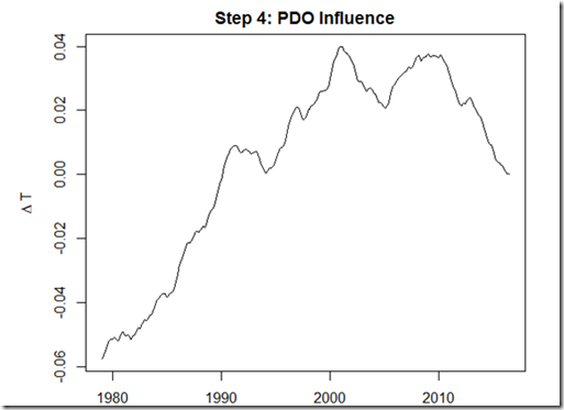
After using this method, we indeed find the “correct” direction for the influence of the PDO:

According to this regression, the warm phase of the PDO contributed about 0.1 K to the warming from 1979-2000, or about 1/3 of the warming over that period. Since shifting to the cool phase at the turn of the 21^st century, it has contributed about 0.04 K cooling to the “hiatus”. This suggests a somewhat smaller influence than England et al. (2014) finds.

For the MMM coefficient, we get a value of 0.73. This would imply that the transient climate sensitivity is biased 37% too high in the multi-model mean. Since the average transient climate sensitivity for CMIP5 is 1.8 K, this coefficient suggests that the TCR should be “adjusted” to 1.3 K. This value corresponds to those found in other observationally-based estimates, most notably Otto et al. (2013).

When we put everything together, and perform the “TCR Adjustment” to the CMIP5 multi-model-mean as well, we get the following result:

 

Conclusion

Using the above methodology, the table below shows the estimated contribution by each factor to the modeled vs. observational temperature discrepancy during the hiatus (note that these rows don’t necessarily add up to 100% since the end result is not a perfect match):

Start Year	Step1: Coverage Bias	Step2: ENSO	Step3: Volc+Solar Forcings	Step4: PDO (surface winds & ocean uptake)	Step5: TCR Bias
1998	36%	10%	17%	2%	28%
1999	45%	0%	23%	6%	35%
2000	39%	9%	23%	7%	28%
2001	31%	16%	20%	5%	21%

According to this method, the coverage bias is responsible for the greatest discrepancy over this period. This is likely contingent upon using Cowtan and Way (2013) rather than simply masking the CMIP5 MMM output (and using HadCRUT4 rather than GISS). Moreover, 65% – 79% of the temperature discrepancy between models and observations during the hiatus may be attributed to something other than a bias in model sensitivity. Nonetheless, this residual warm bias in the multi-model mean does seem to exist, such that the new best estimate for TCR should be closer to 1.3K.

Obviously, there are a number of uncertainties regarding this analysis, and many of these uncertainties may be compounded at each step. Regardless, it seems pretty clear that while the hiatus does not mean that surface warming from greenhouse gases has ceased – given the other factors that may be counteracting such warming in the observed surface temperatures – there is still likely some warm bias in the CMIP5 modeled TCR contributing to the discrepancy.